
Bellman-Ford algorithm stands as a fundamental tool for finding the shortest paths between nodes. Richard Bellman and Lester Ford Jr. founded this algorithm has found applications in computer science. In this article, we will study the Bellman-Ford algorithm along with its code in Python. We will also find its time complexity.
What is Bellman-Ford Algorithm?
Bellman-Ford algorithm is used to find the shortest path from the source vertex to every vertex in a weighted graph. Unlike Dijkstra's algorithm, the Bbellman-Ford algorithm can also find the shortest distance to every vertex in the weighted graph even with the negative edges.
The only difference between the Dijkstra algorithm and the bellman ford algorithm is that Dijkstra's algorithm just visits the neighbor vertex in each iteration but the bellman ford algorithm visits each vertex through each edge in every iteration.
Apart from Bellman-Ford and Dijkstra's, Floyd Warshall Algorithm is also the shortest path algorithm. But the Bellman-Ford algorithm is used to compute the shortest path from the single source vertex to all other vertices whereas Floyd-Warshall algorithms compute the shortest path from each node to every other node.
Here is the simple algorithm:
Begin

   count := 1

   maxEdge := a * (a - 1) / 2     //a is number of vertices


   for all vertices n of the graph, do

      distance[n] := ∞

      pred[n] := ?

   done


   distance[source] := 0

   eCount := number of edges in the graph

   create edge list named edgeList


   while count < a, do

      for k := 0 to eCount, do

         if distance[edgeList[k].n] > distance[edgeList[k].m] + (cost[m,n] for edge k) distance[edgeList[k].n] > distance[edgeList[k].m] + (cost[m,n] for edge k) pred[edgeList[k].n] := edgeList[k].m

      done

   done


   count := count + 1

   for all vertices k in the graph, do

      if distance[edgeList[k].n] > distance[edgeList[k].m] + (cost[m,n] for edge k),

         then return true

   done


   return false

End
Let's look at it step-by-step to understand the Bellman-Ford algorithm:
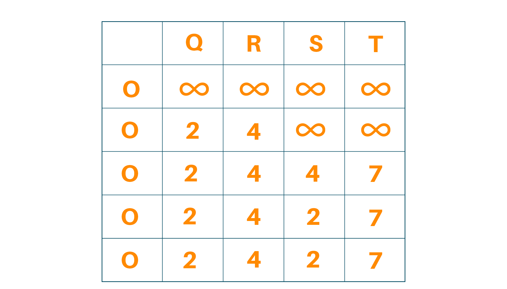
- Initializing the source vertex with distance to itself as 0 and all other vertices as infinity. Creating the array with size N.
- Calculate the shortest distance from the source vertex. Following this process for N-1 times where N is the number of vertices in the graph.
- For relaxing the path lengths for the vertices for each edge m-n:
- if distance[n] > distance[m] + weight of edge mn, then
- distance[n] = distance[m] + weight of edge mn
- Even after minimizing the path lengths for each vertex after N-1 times, if we can still relax the path length where distance[n] > distance[m] + weight of edge mn then we can say that the graph contains the negative edge cycle.
Bellman-Ford algorithm follows the dynamic programming approach by overestimating the length of the path from the starting vertex to all other vertices. And then it starts relaxing the estimates by discovering the new paths which are shorter than the previous ones. This process is followed by all the vertices for N-1 times for finding the optimized result.
Bellman-Ford Algorithm Example
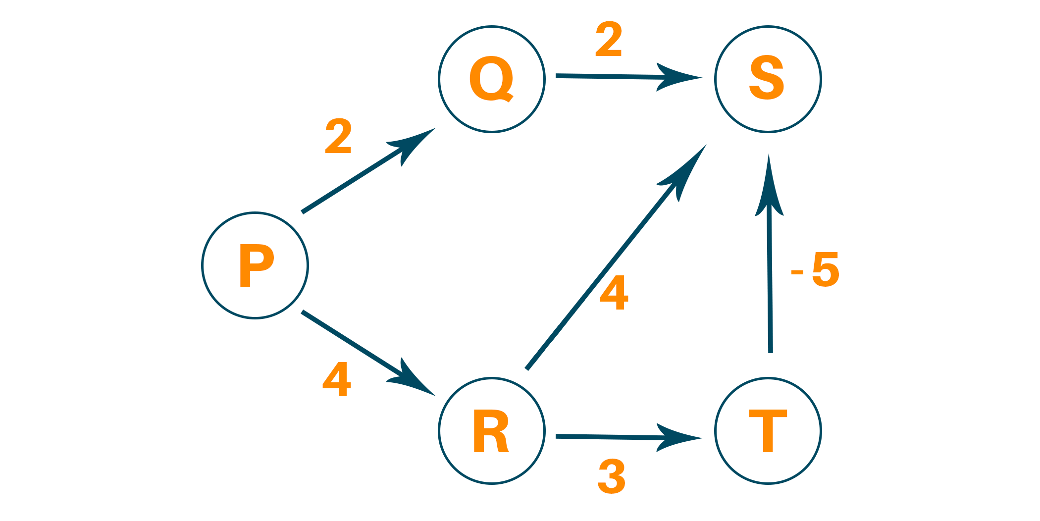
Consider the following weighted graph:
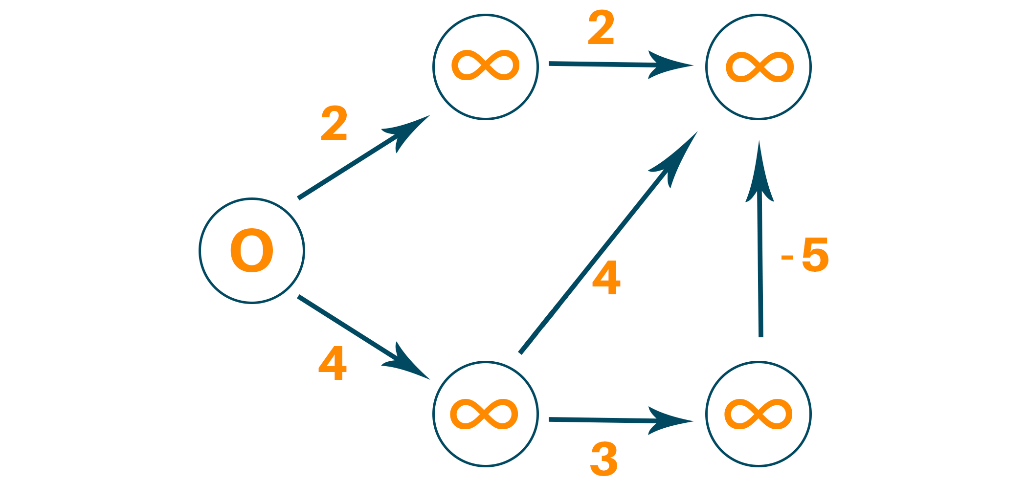
Select the source vertex with path value 0 and all other vertices as infinity.
Visit the neighboring edge from the source vertex and relax the path length of the neighboring vertex if the newly calculated path length is smaller than the previous path length
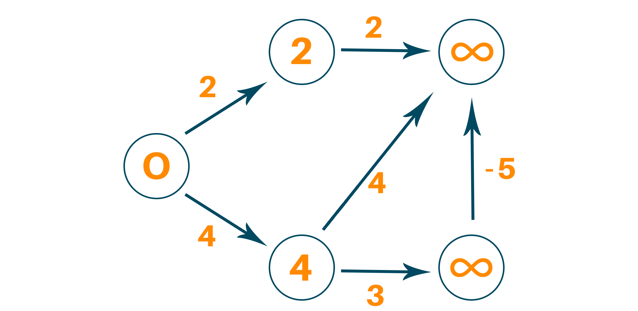
This process must be followed N-1 times where N is the total number of vertices. This is because in the worst-case scenario, any vertex’s path length can be changed to an even smaller path length for N times.
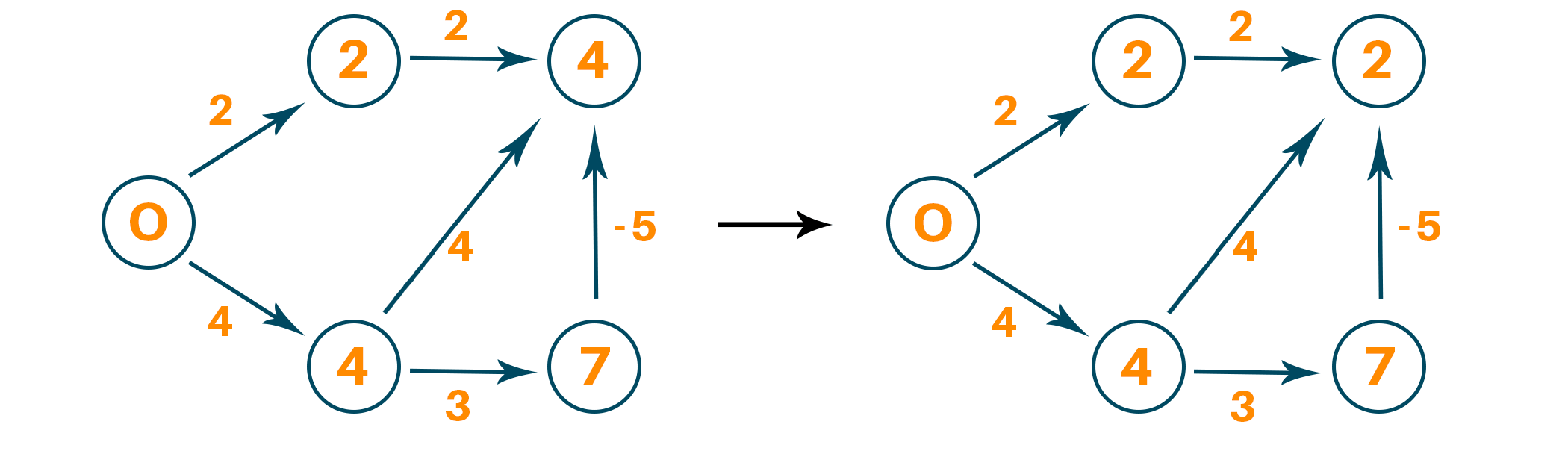
Therefore after N-1 iterations, we find our new path lengths and we can check if the graph has a negative cycle or not.
Look at the following pseudocode:
function bellmanFord(G, S)

  for each vertex N in G

    distance[N] <- infinite

      previous[N] <- NULL

  distance[S] <- 0


  for each vertex N in G

    for each edge (M,N) in G

      tempDistance <- distance[M] + edge_weight(M, N)

      if tempDistance < distance[N]

        distance[N] <- tempDistance

        previous[N] <- M


  for each edge (M,N) in G

    If distance[M] + edge_weight(M, N) < distance[N}

      Error: Negative Cycle Exists


  return distance[], previous[]
We maintain the path length of every vertex and store that in an array with a size N where N is the number of vertices. After the algorithm is over we will backtrack from the last vertex to the source vertex to find the path.
Python Code for Bellman-Ford Algorithm
Here is the full source code to implement the Bellman-Ford algorithm in Python:
class Graph:


    def __init__(self, vertices):

        self.M = vertices   # Total number of vertices in the graph

        self.graph = []     # Array of edges


    # Add edges

    def add_edge(self, a, b, c):

        self.graph.append([a, b, c])


    # Print the solution

    def print_solution(self, distance):

        print("Vertex Distance from Source")

        for k in range(self.M):

            print("{0}\t\t{1}".format(k, distance[k]))


    def bellman_ford(self, src):


        distance = [float("Inf")] * self.M

        distance[src] = 0


        for _ in range(self.M - 1):

            for a, b, c in self.graph:

                if distance[a] != float("Inf") and distance[a] + c < distance[b]:

                    distance[b] = distance[a] + c


        for a, b, c in self.graph:

            if distance[a] != float("Inf") and distance[a] + c < distance[b]:

                print("Graph contains negative weight cycle")

                return


        self.print_solution(distance)


g = Graph(5)

g.add_edge(0, 1, 2)

g.add_edge(0, 2, 4)

g.add_edge(1, 3, 2)

g.add_edge(2, 4, 3)

g.add_edge(2, 3, 4)

g.add_edge(4, 3, -5)


g.bellman_ford(0)
Output:
Vertex Distance from Source
0                   0
1                   2
2                   4
3                   2
4                   7
Time Complexity
The time complexity of the bellman ford algorithm for the best case is O(E) while average-case and worst-case time complexity are O(NE) where N is the number of vertices and E is the total edges to be relaxed. Also, the space complexity of the Bellman-Ford algorithm is O(N) because the size of the array is N.
Is Bellman-Ford better than Dijkstra?
Like everything else, Bellman-Ford and Dijkstra have their own use cases and pros and cons.
The Bellman-Ford algorithm is better in cases where the graph contains non-negative weighted edges. It is designed to handle negative weight edges and can detect negative weight cycles.
This method has a way of handling negative weight edges, but it has a higher time complexity of O(|V|*|E|), where |V| is the number of vertices and |E| is the number of edges. However, in terms of time complexity, Bellman-Ford is less efficient.
On the other hand, for a graph with non-negative edge weights, Dijkstra’s algorithm is a better choice, because it is faster and has better time efficiency. Its time complexity is O((|V| + |E|)log|V|) when using a binary heap priority queue or O(|V|^2) when using a simple array.
Dijkstra’s algorithm is more time efficient because it discards all the paths which are not optimal, ensuring that it takes the shortest possible path.
Where does the Bellman-Ford algorithm fail?
The main purpose of this algorithm is to find the shortest possible path. The presence of a negative-weight cycle can cause the Bellman-Ford algorithm to fail. A negative weight cycle is a cycle in the graph that sums up to a negative weight when the weights of all its edges are added up.
Another case would be if the given graph has no edges since the Bellman-Ford algorithm relies solely on the edges to determine the shortest path. If the graph is a disconnected graph, i.e., if there are no nodes connecting two vertices, the algorithm will malfunction.
Conclusion
In the above article, we studied what is Bellman-Ford algorithm, and understood the Bellman-Ford algorithm step by step along with the example. We further learned Python code and the corresponding output for finding the distance from the source vertex in a weighted graph.