![Machine Learning Algorithms for Beginners [Guide]](https://favtutor.com/resources/images/uploads/machine_learning_Algorithms.jpg)
As a human being can recognize faces and detect images using cognitive skills, with technological advancement, it is now even possible for machines to perform activities that a human can do and even more!
From the beginning of their lives, humans collect data and analyze it to find patterns, our brains are trained in this way to have cognitive skills and interpret data. Likewise, computers can be trained to find a pattern in the data and make appropriate predictions, this is called machine learning. Based on what kind of predictions the models make, there are different machine learning algorithms.
In this guide, we are going to discuss various types of machine learning algorithms for beginners. There are two types of datasets on which algorithms can be trained, one which has prediction or labeled data and another which has only raw data with no actual prediction values to train your model on. The former is a category of supervised learning where your models train on known predictions whereas the latter is unsupervised learning, where the model trains on undetected and unlabeled data. Let’s discuss these algorithms in detail!
Supervised learning
Supervised learning is a category of machine learning algorithms where you have input factors (x) and an output variable (Y) and you utilize an algorithm to create a mapping from the input to the output variable.
Y = f(X)
The objective is to create an efficient and well-defined function that can create predictions as the output on inputting unseen data.
Supervised learning can be further structured into regression and classification problems.
- Regression: It is an algorithm that predicts a continuous real value. Eg. Predicting gold prices. There are many different types of regression algorithms. The three most common are listed below:
- Linear Regression
- Polynomial Regression
- Classification: It is an algorithm that predicts class. Eg. Predicting if the patient is suffering from heart disease or not. Classification problems can be solved with a numerous number of algorithms. Suitable algorithms can be chosen depending upon the data and the structure of the data. Here are a few popular classification algorithms:
- Logistic Regression
- K-Nearest Neighbor
- Support Vector Machines
- Naive Bayes
- Common supervised learning algorithms, which can be used for regression and classification algorithms problems:
- Decision Trees
- Random Forest
Regression Algorithms
Regression problems are unique, as they anticipate that the model should output a real continuous value. For example, predicting stock prices, home loan prices, classifying if the website can be hacked, etc.
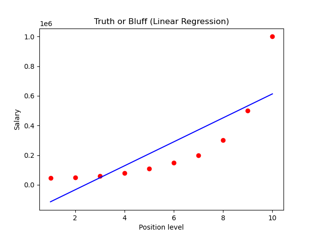
1) Linear Regression
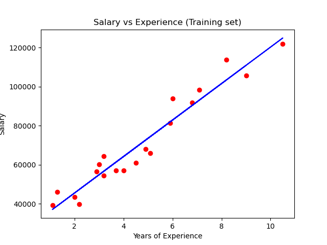
In a simple linear regression algorithm, we create predictions from a single variable. The output attribute is known as the target variable and is alluded to as Y. The input parameter is known as the predictor variable and is alluded to as X. When we consider only one input parameter, the algorithm is known as simple linear regression.
“Linear Regression fits a linear model with coefficients w = (w1, …, wp) to minimize the residual sum of squares between the observed targets in the dataset, and the targets predicted by the linear approximation.”
After creating the test and training data, train the model using scikit learn library.
# Fitting Simple Linear Regression to the Training set
from sklearn.linear_model import LinearRegression
regressor = LinearRegression()
regressor.fit(X_train, y_train)

# Predicting the Test set results
y_pred = regressor.predict(X_test)
The sample plot for the training data following simple linear regression is:
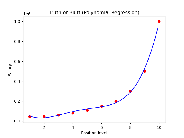
2) Polynomial Regression
In polynomial regression, the input and output variables are mapped in the nth degree of the polynomial. Polynomial Regression doesn't need the connection between the input and output variables to be linear according to the data, this is the basic difference between Linear and Polynomial Regression.
The code below illustrates how you can train a polynomial regression model using python:
# Fitting Linear Regression to the dataset
from sklearn.linear_model import LinearRegression
lin_reg = LinearRegression()
lin_reg.fit(X, y)

# Fitting Polynomial Regression to the dataset
from sklearn.preprocessing import PolynomialFeatures
poly_reg = PolynomialFeatures(degree = 4)
X_poly = poly_reg.fit_transform(X)
poly_reg.fit(X_poly, y)
lin_reg_2 = LinearRegression()
lin_reg_2.fit(X_poly, y)

# Predicting a new result with Linear Regression
lin_reg.predict([[6.5]])
Plots for linear regression and polynomial regression:
Classification Algorithms
3) Logistic regression
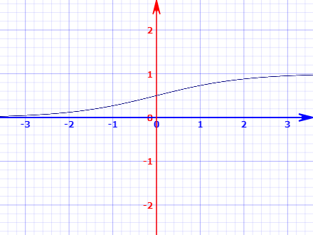
Logistic regression algorithms are used for classification problems. We use a logistic function to generate predictions that is why it is known as Logistic regression.
Another name for the logistic function is the sigmoid function, sigmoid function or activation function is used to convert the output into categorical discrete value. It’s an S-shaped curve that inputs a real-valued number and maps it into a value between 0 and 1. The logistic regression equation is:
1/(1 + e-value)
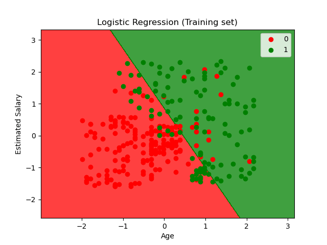
After creating and scaling the training and test dataset we can fit our training data to the model and create model predictions on the test data. And create a confusion matrix.
# Feature Scaling
from sklearn.preprocessing import StandardScaler
sc = StandardScaler()
X_train = sc.fit_transform(X_train)
X_test = sc.transform(X_test)

# Fitting Logistic Regression to the Training set
from sklearn.linear_model import LogisticRegression
classifier = LogisticRegression(random_state = 0)
classifier.fit(X_train, y_train)

# Predicting the Test set results
y_pred = classifier.predict(X_test)

# Making the Confusion Matrix
from sklearn.metrics import confusion_matrix
cm = confusion_matrix(y_test, y_pred)
The decision boundary and scatter plot for the training data predicting if the user will purchase the commodity based on the data from social media advertisement, looks like this:
The model can overfit if the input parameters are highly correlated like linear regression, to cure this we can map pairwise correlations between inputs by removing the highly correlated inputs.
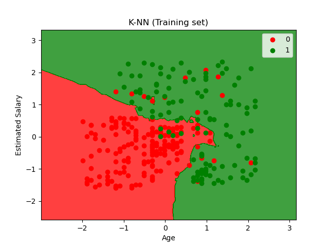
4) K-Nearest Neighbor algorithm
KNN is used for both regression and classification problems. However, it is vastly used for classification problems. K-nearest neighbors (KNN) algorithm uses ‘feature similarity’ to create the prediction values of new data points. This implies that new data points are assigned new values based on points in the training set. The working of the algorithm-
- Step 1: Creating training and test data.
- Step 2: We choose the value of K i.e. the nearest data points. K can be any integer. N− For each point in the test data do the following:
- 2.1: Calculate the distance between test data and each value of training data using any of the methods namely: Euclidean, Manhattan, or Hamming distance. Euclidean distance is the most common method.
- 2.2: Sort the distance in ascending order.
- 2.3: The algorithm chooses the top K rows from the sorted array.
- 2.4: It will assign a class to the test point based on the most frequent class of these rows.
The training data is fit into the KNN model and predictions are created using test data and create confusion matrix:
# Feature Scaling
from sklearn.preprocessing import StandardScaler
sc = StandardScaler()
X_train = sc.fit_transform(X_train)
X_test = sc.transform(X_test)

# Fitting K-NN to the Training set
from sklearn.neighbors import KNeighborsClassifier
classifier = KNeighborsClassifier(n_neighbors = 5, metric = 'minkowski', p = 2)
classifier.fit(X_train, y_train)

# Predicting the Test set results
y_pred = classifier.predict(X_test)

# Making the Confusion Matrix
from sklearn.metrics import confusion_matrix
cm = confusion_matrix(y_test, y_pred)
The plot of the training data and labels with decision boundary according to the KNN classification algorithm:
5) Support Vector machines - Kernel SVM
The aim of support vector machine algorithms is to find a hyperplane in an N-dimensional space where N is the number of features that are used to distinctly classify data.
There are many different methods or hyperplanes to separate the two classes of data points. Our aim is to find a hyperplane with a maximum distance between data points of both classes. Maximizing the margin distance enhances the efficiency of the model and predicts with more confidence.
The code to scale and fit the training data is:
# Feature Scaling
from sklearn.preprocessing import StandardScaler
sc = StandardScaler()
X_train = sc.fit_transform(X_train)
X_test = sc.transform(X_test)

# Fitting Kernel SVM to the Training set
from sklearn.svm import SVC
classifier = SVC(kernel = 'rbf', random_state = 0)
classifier.fit(X_train, y_train)

# Predicting the Test set results
y_pred = classifier.predict(X_test)

# Making the Confusion Matrix
from sklearn.metrics import confusion_matrix
cm = confusion_matrix(y_test, y_pred)
The plot of the training data and labels with decision boundary according to the SVM classification algorithm:

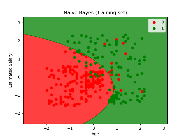
6) Naïve Bayes Algorithm
Naïve Bayes Classifier is one of the straightforward and best Classification algorithms which helps in building the fast machine learning models which will make quick predictions.
It is a probabilistic classifier, which suggests it predicts the idea of the probability of an object. Some popular examples of the Naïve Bayes Algorithm are spam filters, sentimental analysis, and classifying articles.
The algorithm follows the following equation:
P(h|d) = (P(d|h) * P(h)) / P(d)
And this is how we fit the data to the naive Bayes model:
# Fitting Naive Bayes to the Training set
from sklearn.naive_bayes import GaussianNB
classifier = GaussianNB()
classifier.fit(X_train, y_train)

# Predicting the Test set results
y_pred = classifier.predict(X_test)

# Making the Confusion Matrix
from sklearn.metrics import confusion_matrix
cm = confusion_matrix(y_test, y_pred)
Naive Bayes is often extended to real-valued attributes, most ordinarily by assuming a normal distribution.
This extension of naive Bayes is named Gaussian Naive Bayes. The Gaussian (or Normal distribution) is the easiest method because we only need to estimate the mean and therefore the variance from our training data.
The plot of decision boundary for a gaussian naive Bayes algorithm on training data:
Common Supervised learning Algorithms
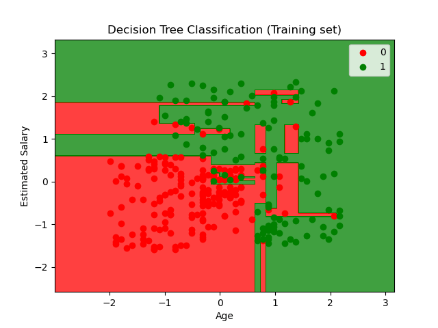
7) Decision Tree Algorithm
The decision tree as the name suggests works on the principle of conditions. It is efficient and has strong algorithms used for predictive analysis. It has mainly attributed that include internal nodes, branches, and a terminal node.
Every internal node holds a “test” on an attribute, branches hold the conclusion of the test and every leaf node means the class label. It is used for both classifications as well as regression which are both supervised learning algorithms. Decisions trees are extremely delicate to the information they are prepared on — little changes to the preparation set can bring about fundamentally different tree structures.
Trees answer consecutive roles that send us down a specific use of the tree given we have the answer. The model acts with "if this then that" conditions, at last, yielding a particular outcome. The code to fit the training data to the decision tree classification model:
# Feature Scaling
from sklearn.preprocessing import StandardScaler
sc = StandardScaler()
X_train = sc.fit_transform(X_train)
X_test = sc.transform(X_test)

# Fitting Decision Tree Classification to the Training set
from sklearn.tree import DecisionTreeClassifier
classifier = DecisionTreeClassifier(criterion = 'entropy', random_state = 0)
classifier.fit(X_train, y_train)

# Predicting the Test set results
y_pred = classifier.predict(X_test)

# Making the Confusion Matrix
from sklearn.metrics import confusion_matrix
cm = confusion_matrix(y_test, y_pred)
The plot showing the decision boundary for the decision tree classification algorithm for the training data.
8) Random Forest Algorithm
Random forest, as its name suggests, comprises an enormous amount of individual decision trees that work as a group or as they say, an ensemble. Every individual decision tree in the random forest lets out a class prediction and the class with the most votes is considered as the model's prediction.
Random forest uses this by permitting every individual tree to randomly sample from the dataset with replacement, bringing about various trees. This is known as bagging. You can refer to a detailed tutorial on Random forest classifier by making a project on credit card fraud detection using machine learning.
Fitting the training data:
# Feature Scaling
from sklearn.preprocessing import StandardScaler
sc = StandardScaler()
X_train = sc.fit_transform(X_train)
X_test = sc.transform(X_test)

# Fitting Random Forest Classification to the Training set
from sklearn.ensemble import RandomForestClassifier
classifier = RandomForestClassifier(n_estimators = 10, criterion = 'entropy', random_state = 0)
classifier.fit(X_train, y_train)

# Predicting the Test set results
y_pred = classifier.predict(X_test)

# Making the Confusion Matrix
from sklearn.metrics import confusion_matrix
cm = confusion_matrix(y_test, y_pred)
The plot for the training data for the random forest classification. You can notice that the plot somewhat looks like the plot for the decision tree but with better accuracy of the decision boundary.

Unsupervised Learning
An unsupervised learning algorithm is training a model on data that is neither classified nor labeled and allowing the algorithm to find patterns in the data without guidance. The algorithm groups the unsorted information according to patterns without any prior training of the model on any data.
Unlike supervised learning, no labels are provided in the data that means no training is done for the model. Therefore models are restricted to find the hidden structure in unlabeled data by our-self.
In this guide, we’ll discuss the two most prominent unsupervised learning algorithms, namely K-mean clustering and Principal component analysis.
9) K-means clustering Algorithm
K-Means Clustering is an Unsupervised Learning algorithm, which groups the unlabeled dataset into different clusters. Here K is the number of predefined clusters that are needed to train the model, as if K=2, there will be two clusters, and for K=3, there will be three clusters, and so on.
“It is an iterative algorithm that divides the unlabeled dataset into k different clusters in such a way that each dataset belongs to only one group that has similar properties.”
To choose the optimal number of clusters for the model, we use the elbow method:
- It trains the K-means clustering model on the given dataset with different K values (ranges from 1-10).
- For each value of K, calculate the WCSS value.
- The plot between calculated WCSS values and the number of clusters K.
- The steep bend or a point of the plot looks like an arm, that point is considered as the best value of K.
The WCSS curve looks like this:
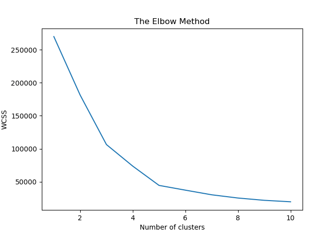
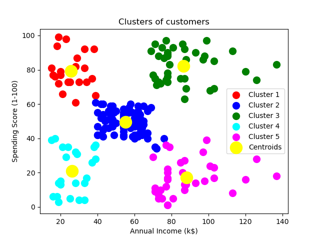
From the curve, we deduce that the most suitable number of clusters (K) is 5. Hence the code to fit an unlabeled data by finding the number of clusters using the elbow method to a K-mean clustering model is:
# Using the elbow method to find the optimal number of clusters
from sklearn.cluster import KMeans
wcss = []
for i in range(1, 11):
    kmeans = KMeans(n_clusters = i, init = 'k-means++', random_state = 42)
    kmeans.fit(X)
    wcss.append(kmeans.inertia_)
plt.plot(range(1, 11), wcss)
plt.title('The Elbow Method')
plt.xlabel('Number of clusters')
plt.ylabel('WCSS')
plt.show()

# Fitting K-Means to the dataset
kmeans = KMeans(n_clusters = 5, init = 'k-means++', random_state = 42)
y_kmeans = kmeans.fit_predict(X)
The number of clusters and the data segmentation and centroid of the clusters created by the model is:
10) Principal Component Analysis
The main purpose of PCA is to decrease the complexity of the model. PCA simplifies the model and improves model performance. In cases of the datasets which have a lot of features we just extract much fewer independent variables that explain the variance the most.
The principal component analysis is used to extract linear composites of the observed variables. Factor analysis is basically a formal model predicting observed variables from theoretical latent factors from the dataset. We use PCA to maximize the total variance to find distinguishable patterns, and Factor analysis to maximize the shared variance for latent constructs or variables.
Reinforcement Learning
Reinforcement learning is used to make a sequence of decisions. The model learns to achieve a goal for an uncertain, potentially complex dataset. The concept of reinforcement learning is very similar to a game. The model uses a trial and error method to solve the problem. To achieve the goal the model gets either rewards or penalties for the actions it performs. Its primary goal of the model is to maximize the total reward.
There are two types of Reinforcement:
Positive Reinforcement
It is when an event occurs due to a particular behavior and resulting in an increase in the strength and the frequency of the behavior. Consequently, it has a positive effect on the behavior of the model.
Advantages of reinforcement learning are:
- Maximizes Performance
- Sustain Change for a long period of time
Disadvantages of reinforcement learning:
- Too much Reinforcement can lead to an overload of states which can diminish the results.
Negative Reinforcement
It is defined as the strengthening of behavior because a negative condition is stopped or avoided.
Advantages of reinforcement learning:
- Increases Behavior
- Provide defiance to a minimum standard of performance
Disadvantages of reinforcement learning:
- It facilitates enough to meet up the minimum behavior
Conclusion
Now that you know all about machine learning algorithms, you can start working with machine learning projects to apply your knowledge to real-world problems.
Machine learning is all about handling and processing the data and speculating the best machine learning algorithm to train your model to get optimal results. Python libraries like scikit-learn make it pretty easy to train your data without working out the actual mathematics behind the machine learning algorithm but understanding the algorithm to its core is what makes you a good data scientist.
We have covered 10 of the most prominent machine learning algorithms for beginners in this tutorial. Hope this article helps you create a clear understanding of the buzzword nowadays. That’s right Machine Learning.
Happy Learning :)