

Logistic Regression is a classifier that belongs to the class of linear models. Mathematically, it is a sigmoid transformation of the fitted equation of a line (in n-dimensions where n is the number of features taken into account) that denotes the class probabilities absolutely suitable for Binary Classification after a proper thresholding is done. This line is known as Decision Boundary which is a boundary line created by the classifier (here, Logistic Regression) to signify the decision regions. The visualization of decision boundary along with the data-points (colored data-points to describe the respective labeled classes) is difficult if the data is more than 2-3 dimensions. In this article, Decision Boundary Visualization is performed by training a Logistic Regression Model on the Breast Cancer Wisconsin (Diagnostic) Data Set after applying Principal Component Analysis on the same in order to reduce the number of dimensions of the dataset to 2 dimensions.
15 Steps to Generate Decision Boundary Visualization
1. Importing necessary libraries
# importing necessary libraries
import numpy as np
import pandas as pd
pd.set_option("display.max_rows", None, "display.max_columns", None) # displaying all rows and columns of a dataframe
from sklearn.model_selection import train_test_split
from sklearn.preprocessing import StandardScaler
from sklearn.decomposition import IncrementalPCA
from sklearn.model_selection import GridSearchCV
from sklearn.linear_model import LogisticRegression
from sklearn import metrics
import matplotlib.pyplot as plt
import seaborn as sns
%matplotlib inline
2. Reading the Breast Cancer Wisconsin (Diagnostic) Dataset
The Breast Cancer Wisconsin (Diagnostic) Dataset is obtained from Kaggle (https://www.kaggle.com/uciml/breast-cancer-wisconsin-data) and is originally available at the UCI Data Repository.
# reading the Breast Cancer Wisconsin (Diagnostic) Data Set
df = pd.read_csv('data.csv')

# displaying top 5 instances of the dataset
print(df.head())
Corresponding Output
         id diagnosis  radius_mean  texture_mean  perimeter_mean  area_mean  \
0    842302         M        17.99         10.38          122.80     1001.0
1    842517         M        20.57         17.77          132.90     1326.0
2  84300903         M        19.69         21.25          130.00     1203.0
3  84348301         M        11.42         20.38           77.58      386.1
4  84358402         M        20.29         14.34          135.10     1297.0

   smoothness_mean  compactness_mean  concavity_mean  concave points_mean  \
0          0.11840           0.27760          0.3001              0.14710
1          0.08474           0.07864          0.0869              0.07017
2          0.10960           0.15990          0.1974              0.12790
3          0.14250           0.28390          0.2414              0.10520
4          0.10030           0.13280          0.1980              0.10430

   symmetry_mean  fractal_dimension_mean  radius_se  texture_se  perimeter_se  \
0         0.2419                 0.07871     1.0950      0.9053         8.589
1         0.1812                 0.05667     0.5435      0.7339         3.398
2         0.2069                 0.05999     0.7456      0.7869         4.585
3         0.2597                 0.09744     0.4956      1.1560         3.445
4         0.1809                 0.05883     0.7572      0.7813         5.438

   area_se  smoothness_se  compactness_se  concavity_se  concave points_se  \
0   153.40       0.006399         0.04904       0.05373            0.01587
1    74.08       0.005225         0.01308       0.01860            0.01340
2    94.03       0.006150         0.04006       0.03832            0.02058
3    27.23       0.009110         0.07458       0.05661            0.01867
4    94.44       0.011490         0.02461       0.05688            0.01885

   symmetry_se  fractal_dimension_se  radius_worst  texture_worst  \
0      0.03003              0.006193         25.38          17.33
1      0.01389              0.003532         24.99          23.41
2      0.02250              0.004571         23.57          25.53
3      0.05963              0.009208         14.91          26.50
4      0.01756              0.005115         22.54          16.67

   perimeter_worst  area_worst  smoothness_worst  compactness_worst  \
0           184.60      2019.0            0.1622             0.6656
1           158.80      1956.0            0.1238             0.1866
2           152.50      1709.0            0.1444             0.4245
3            98.87       567.7            0.2098             0.8663
4           152.20      1575.0            0.1374             0.2050

   concavity_worst  concave points_worst  symmetry_worst  \
0           0.7119                0.2654          0.4601
1           0.2416                0.1860          0.2750
2           0.4504                0.2430          0.3613
3           0.6869                0.2575          0.6638
4           0.4000                0.1625          0.2364

   fractal_dimension_worst  Unnamed: 32
0                  0.11890          NaN
1                  0.08902          NaN
2                  0.08758          NaN
3                  0.17300          NaN
4                  0.07678          NaN
3. Dropping unwanted columns, 'id' and 'Unnamed: 32' are dropped
# the unwanted columns, 'id' and 'Unnamed: 32' are dropped
df.drop(['id', 'Unnamed: 32'], axis = 1, inplace = True)
4. Label Encoding of the Target Variable
# label-encoding of the target label, 'diagnosis' such that B(Benign) -> 0 and M (Malignant) -> 1
df['diagnosis'] = df['diagnosis'].map({'B':0, 'M':1})
5. Creating the Feature Set and Target Label variables
# spliting into X (features) and y (target label)
X = df.iloc[:, 1:]
y = df['diagnosis']
6. 80-20 splitting the dataset into Training Set and Test Set
# 80-20 splitting into train and test sets
X_train, X_test, y_train, y_test = train_test_split(X, y,
                                                    train_size = 0.8,
                                                    test_size = 0.2, random_state = 1234)
7. Feature Scaling of the features in the Training and Test Set
# feature scaling of the features in Training and Test Set
columns = X_train.columns
scalerx = StandardScaler()
X_train_scaled = scalerx.fit_transform(X_train)
X_train_scaled = pd.DataFrame(X_train_scaled, columns = columns)

X_test_scaled = scalerx.transform(X_test)
X_test_scaled = pd.DataFrame(X_test_scaled, columns = columns)
8. Principal Component Analysis (PCA) to reduce the dimensionality of the data into 2 dimensions in both Training and Test Set
# Incremental Principal Component Analysis to select 2 features such that they explain as much variance as possible
pca = IncrementalPCA(n_components = 2)
X_train_pca = pca.fit_transform(X_train_scaled)

X_test_pca = pca.transform(X_test_scaled)
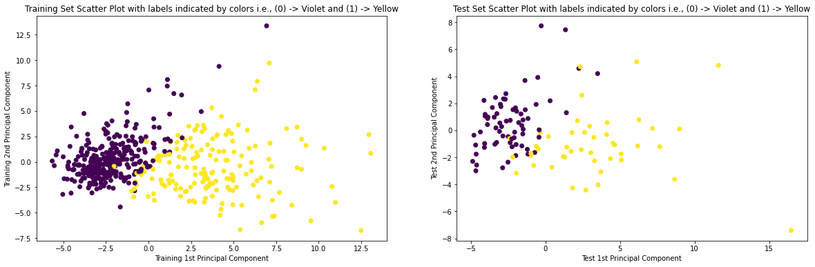
9. Plotting the Scatter-Plot of Training and Test Set
# Scatter Plot of Training and Test Set with labels indicated by colors
plt.figure(figsize = (20, 6))
plt.subplot(1, 2, 1)
plt.scatter(X_train_pca[:,0], X_train_pca[:,1], c = y_train)
plt.xlabel('Training 1st Principal Component')
plt.ylabel('Training 2nd Principal Component')
plt.title('Training Set Scatter Plot with labels indicated by colors i.e., (0) -> Violet and (1) -> Yellow')
plt.subplot(1, 2, 2)
plt.scatter(X_test_pca[:,0], X_test_pca[:,1], c = y_test)
plt.xlabel('Test 1st Principal Component')
plt.ylabel('Test 2nd Principal Component')
plt.title('Test Set Scatter Plot with labels indicated by colors i.e., (0) -> Violet and (1) -> Yellow')
plt.show()
Corresponding Output
10. Performing 5-Fold Grid-Search Cross Validation on Logistic Regression Classifier on the Training Set
# 5-Fold Grid-Search Cross Validation on Logistic Regression Classifier for tuning the hyper-parameter, C with Accuracy scoring
params = {'C':[0.01, 0.1, 1, 10, 100]}

clf = LogisticRegression()

folds = 5
model_cv = GridSearchCV(estimator = clf,
                        param_grid = params,
                        scoring= 'accuracy',
                        cv = folds,
                        return_train_score=True,
                        verbose = 3)

model_cv.fit(X_train_pca, y_train)
Corresponding Output
Fitting 5 folds for each of 5 candidates, totalling 25 fits
[CV 1/5] END .........................................C=0.01; total time=   0.0s
[CV 2/5] END .........................................C=0.01; total time=   0.0s
[CV 3/5] END .........................................C=0.01; total time=   0.0s
[CV 4/5] END .........................................C=0.01; total time=   0.0s
[CV 5/5] END .........................................C=0.01; total time=   0.0s
[CV 1/5] END ..........................................C=0.1; total time=   0.0s
[CV 2/5] END ..........................................C=0.1; total time=   0.0s
[CV 3/5] END ..........................................C=0.1; total time=   0.0s
[CV 4/5] END ..........................................C=0.1; total time=   0.0s
[CV 5/5] END ..........................................C=0.1; total time=   0.0s
[CV 1/5] END ............................................C=1; total time=   0.0s
[CV 2/5] END ............................................C=1; total time=   0.0s
[CV 3/5] END ............................................C=1; total time=   0.0s
[CV 4/5] END ............................................C=1; total time=   0.0s
[CV 5/5] END ............................................C=1; total time=   0.0s
[CV 1/5] END ...........................................C=10; total time=   0.0s
[CV 2/5] END ...........................................C=10; total time=   0.0s
[CV 3/5] END ...........................................C=10; total time=   0.0s
[CV 4/5] END ...........................................C=10; total time=   0.0s
[CV 5/5] END ...........................................C=10; total time=   0.0s
[CV 1/5] END ..........................................C=100; total time=   0.0s
[CV 2/5] END ..........................................C=100; total time=   0.0s
[CV 3/5] END ..........................................C=100; total time=   0.0s
[CV 4/5] END ..........................................C=100; total time=   0.0s
[CV 5/5] END ..........................................C=100; total time=   0.0s
GridSearchCV(cv=5, estimator=LogisticRegression(),
             param_grid={'C': [0.01, 0.1, 1, 10, 100]}, return_train_score=True,
             scoring='accuracy', verbose=3)
11. Getting the Best Hyper-parameter from the Grid-Search performed above
# getting the best hyper-parameter
print(model_cv.best_params_)
Corresponding Output
{'C': 10}
12. Re-training the Logistic Regression Classifier with the best hyper-parameter, C = 10 (obtained above)
# re-training the Logistic Regression Classifier with the best hyper-parameter, C = 10
model = LogisticRegression(C = 10).fit(X_train_pca, y_train)
13. Obtaining the Training Set and Test Set Predictions given by the model, trained in the last step
# getting the Training Set Predictions
y_train_pred = model.predict(X_train_pca)

# getting the Test Set Predictions
y_test_pred = model.predict(X_test_pca)
14. Performance Analysis of the Logistic Regression Model in terms of Accuracy, Precision, Recall and F1-Score
# Getting the Training and Test Accuracy of the Logistic Regression Model
print('Training Accuracy of the Model: ', metrics.accuracy_score(y_train, y_train_pred))
print('Test Accuracy of the Model: ', metrics.accuracy_score(y_test, y_test_pred))
print()

# Getting the Training and Test Precision of the Logistic Regression Model
print('Training Precision of the Model: ', metrics.precision_score(y_train, y_train_pred))
print('Test Precision of the Model: ', metrics.precision_score(y_test, y_test_pred))
print()

# Getting the Training and Test Recall of the Logistic Regression Model
print('Training Recall of the Model: ', metrics.recall_score(y_train, y_train_pred))
print('Test Recall of the Model: ', metrics.recall_score(y_test, y_test_pred))
print()

# Getting the Training and Test F1-Score of the Logistic Regression Model
print('Training F1-Score of the Model: ', metrics.f1_score(y_train, y_train_pred))
print('Test F1-Score of the Model: ', metrics.f1_score(y_test, y_test_pred))
print()
Corresponding Output
Training Accuracy of the Model:  0.9648351648351648
Test Accuracy of the Model:  0.9035087719298246

Training Precision of the Model:  0.9520958083832335
Test Precision of the Model:  0.9473684210526315

Training Recall of the Model:  0.9520958083832335
Test Recall of the Model:  0.8

Training F1-Score of the Model:  0.9520958083832335
Test F1-Score of the Model:  0.8674698795180723
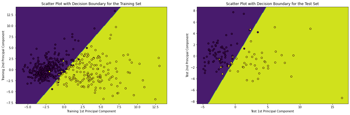
15. Plotting the Decision Boundary given by the Trained Logistic Regression both on the Training and Test sets
# plotting the decision boundary in the scatter plot of Training and Test Set with labels indicated by colors
x_min, x_max = X_train_pca[:, 0].min() - 1, X_train_pca[:, 0].max() + 1
y_min, y_max = X_train_pca[:, 1].min() - 1, X_train_pca[:, 1].max() + 1

xx_train, yy_train = np.meshgrid(np.arange(x_min, x_max, 0.1),
                                 np.arange(y_min, y_max, 0.1))

Z_train = model.predict(np.c_[xx_train.ravel(), yy_train.ravel()])
Z_train = Z_train.reshape(xx_train.shape)


x_min, x_max = X_test_pca[:, 0].min() - 1, X_test_pca[:, 0].max() + 1
y_min, y_max = X_test_pca[:, 1].min() - 1, X_test_pca[:, 1].max() + 1

xx_test, yy_test = np.meshgrid(np.arange(x_min, x_max, 0.1),
                               np.arange(y_min, y_max, 0.1))

Z_test = model.predict(np.c_[xx_test.ravel(), yy_test.ravel()])
Z_test = Z_test.reshape(xx_test.shape)


plt.figure(figsize = (20, 6))
plt.subplot(1, 2, 1)
plt.contourf(xx_train, yy_train, Z_train)
plt.scatter(X_train_pca[:, 0], X_train_pca[:, 1], c = y_train, s = 30, edgecolor = 'k')
plt.xlabel('Training 1st Principal Component')
plt.ylabel('Training 2nd Principal Component')
plt.title('Scatter Plot with Decision Boundary for the Training Set')
plt.subplot(1, 2, 2)
plt.contourf(xx_test, yy_test, Z_test)
plt.scatter(X_test_pca[:, 0], X_test_pca[:, 1], c = y_test, s = 30, edgecolor = 'k')
plt.xlabel('Test 1st Principal Component')
plt.ylabel('Test 2nd Principal Component')
plt.title('Scatter Plot with Decision Boundary for the Test Set')
plt.show()
Corresponding Output
Conclusion
So, from the Decision Boundaries generated above, it can be re-interpreted and re-established that Logistic Regression Classifier belongs to the class of linear models. Apart from that, it can also be concluded that in addition to Performance Metrics like Accuracy, Precision, Recall and F1-Score, Decision Boundary is a visual representation of the Model Performance as well.


.png)