
The 0-1 Knapsack Problem is a classic combinatorial optimization problem in the field of computer science and mathematics. In this article, we will discuss the 0/1 Knapsack Problem, along with examples. The benefits, drawbacks, and uses of the 0/1 knapsack issue will also be covered in this last section. Therefore, let's begin!
What is the 0-1 Knapsack Problem?
Imagine you have a backpack that can only hold a certain amount of weight. You have a bunch of toys that you want to take with you on a trip, but you can't take all of them because they won't fit in your backpack.
The 0/1 knapsack problem is like trying to decide which toys to bring with you. You have to choose which toys you want to bring and which toys you want to leave behind. The twist is that each toy has a different weight and value. Some toys are heavier than others, but they may also be more valuable.
The goal is to fill up your backpack with the toys that will give you the most value without making your backpack too heavy. It's like a puzzle where you have to figure out the best combination of toys to bring with you.
Formally speaking, the problem can be stated as follows:
Given a set of N items, each with a weight w(i) and a value v(i), and a knapsack with a maximum weight capacity W, select a subset of the items to include in the knapsack, such that the total weight of the selected items does not exceed W, and the total value of the selected items is maximized.
In this problem, the decision variable for each item is binary, meaning that each item can either be included in the knapsack (1) or not (0). Thus, the problem is also known as the "binary knapsack problem".
The problem can be modeled mathematically using the following objective function:
maximize: ∑(i=1 to N) v(i)x(i)
subject to: ∑(i=1 to N) w(i)x(i) <= W
x(i) = {0,1} for i = 1,2,..N
where x(i) is a binary decision variable that takes a value of 1 if the item i is selected to be included in the knapsack, and 0 otherwise.
The objective function maximizes the total value of the selected items, while the constraint ensures that the total weight of the selected items does not exceed the maximum weight capacity of the knapsack.
The 0/1 Knapsack Problem is a combinatorial optimization problem, which means that there are a large number of possible combinations of items that can be selected to fill the knapsack. The problem is known to be NP-hard, which means that there is no known polynomial-time algorithm to find an exact solution for large instances of the problem.
Therefore, various approximate algorithms and heuristics are used to solve the problem, including dynamic programming, branch and bound, and genetic algorithms, among others. These algorithms can provide good solutions to the problem, although they may not always guarantee an optimal solution.
The most basic way to solve the 0/1 knapsack problem is using recursion. Let's take a look at the algorithm for doing so:
Input:
- weights: an array of item weights
- values: an array of item values
- i: the index of the current item
- j: the remaining knapsack capacity
Output:
The maximum value that can be obtained with the given items and knapsack capacity.
- If there are no items left or the remaining knapsack capacity is zero, return 0.
- If the weight of the current item is greater than the remaining knapsack capacity, skip the current item and move on to the next item. Return the result of recursively calling the knapsack with the remaining items and the same knapsack capacity.
- Otherwise, we have two options: include the current item or skip it. Return the maximum value obtained by:
- Including the current item: add the value of the current item to the result of recursively calling the knapsack with the remaining items and the remaining knapsack capacity (i.e., subtracting the weight of the current item from the remaining capacity).
- Skipping the current item: return the result of recursively calling the knapsack with the remaining items and the same knapsack capacity.
The base case for the recursion is when there are no items left or the remaining knapsack capacity is zero. In this case, the function returns 0, as there is no more value to be gained.
The recursive algorithm explores all possible combinations of items that can be included in the knapsack, starting with the last item and moving backward. The function selects the item with the highest value that can be included without exceeding the knapsack capacity.
Note that this algorithm has a time complexity of O(2^n), where n is the number of items since it explores all possible combinations of items. This makes it inefficient for large input sizes, and dynamic programming approaches are usually used to solve the 0/1 knapsack problem more efficiently.
Here is the C++ code for the 0/1 knapsack problem:
#include
#include
using namespace std;

int knapsack(vector<int>& weights, vector<int>& values, int i, int j) {
    if (i == 0 || j == 0) {
        return 0;
    }
    if (weights[i-1] > j) {
        return knapsack(weights, values, i-1, j);
    } else {
        return max(values[i-1] + knapsack(weights, values, i-1, j-weights[i-1]),
                   knapsack(weights, values, i-1, j));
    }
}

int main() {
    vector<int> weights = {2,3, 4, 5};
    vector<int> values = {10, 20, 50, 60};
    int capacity = 8;
    int max_value = knapsack(weights, values, weights.size(), capacity);
    cout << "Maximum value: " << max_value << endl;
    return 0;
}
Output:
Maximum value: 80
Time Complexity: O(2^N)
Space Complexity: O(N), Required Stack Space for Recursion
In this code, weights is a vector of item weights, values is a vector of item values, i is the index of the current item, and j is the current knapsack capacity. The function returns the maximum value that can be obtained with the given items and knapsack capacity.
The base cases are when either there are no items left or the knapsack capacity is zero, in which case the maximum value is zero.
If the weight of the current item is greater than the remaining knapsack capacity, the current item cannot be included in the knapsack, so we move on to the next item by calling knapsack(weights, values, i-1, j).
Otherwise, we have two options: include the current item and reduce the remaining capacity by its weight, or exclude the current item and move on to the next item. We choose the option that gives us the maximum value by calling max(values[i-1] + knapsack(weights, values, i-1, j-weights[i-1]), knapsack(weights, values, i-1, j)).
To use this function, you can create vectors for the item weights and values, set the knapsack capacity, and call the knapsack function with the vectors and capacity as arguments.
Equivalent Python code for the same problem:
def knapsack(weights, values, i, j):
    if i == 0 or j == 0:
        return 0
    if weights[i-1] > j:
        return knapsack(weights, values, i-1, j)
    else:
        return max(values[i-1] + knapsack(weights, values, i-1, j-weights[i-1]),
                   knapsack(weights, values, i-1, j))

# Example usage
weights = [2, 3, 4, 5]
values = [10, 20, 50, 60]
capacity = 8
max_value = knapsack(weights, values, len(weights), capacity)
print("Maximum value:", max_value)
Output:
Maximum value: 80
Time Complexity: O(2^N)
Space Complexity: O(N), Required Stack Space for Recursion
Advantages
- It is a well-known and well-studied problem, and there are efficient algorithms to solve it. For example, dynamic programming can solve the problem in O(N*W) time, where n is the number of items and W is the maximum weight capacity of the knapsack.
- The problem has many real-world applications, such as resource allocation, project selection, and financial portfolio management.
- The problem can be extended to the case where items can be split and placed in the knapsack partially, which leads to the fractional knapsack problem.
Disadvantages
- The 0/1 Knapsack problem is an NP-hard problem, which means that there is no known polynomial time algorithm that can solve it for all cases.
- The problem assumes that the values and weights of the items are known beforehand, which may not be the case in some real-world scenarios.
- The problem does not take into account any constraints other than the weight capacity of the knapsack, such as budget constraints or time constraints.
Applications
- Resource allocation: The problem can be used to allocate limited resources such as manpower, equipment, or materials to different projects or tasks while maximizing the overall value or profit.
- Financial portfolio management: The problem can be used to select a portfolio of financial assets with limited investment funds while maximizing the expected return or minimizing the risk.
- Cutting stock problem: The problem can be used to minimize the amount of waste material when cutting large sheets of material such as wood, glass, or metal into smaller pieces of various sizes.
- Project selection: The problem can be used to select a set of projects to invest in, with limited resources and time, while maximizing the overall profit or benefit.
- Knapsack packing: The problem can be used to pack a set of items of various shapes and sizes into a container of limited capacities, such as a backpack, a shipping container, or a warehouse.
- DNA sequencing: The problem can be used to assemble a sequence of DNA fragments of varying lengths and weights while minimizing the overall sequencing cost.
Knapsack Problem Example
Moving on, let's fixate on a 0/1 knapsack problem example that will help us with further concepts:
Let's consider we have 4 objects, for each object, there's some weight and value associated with it. There's a knapsack of capacity 8.
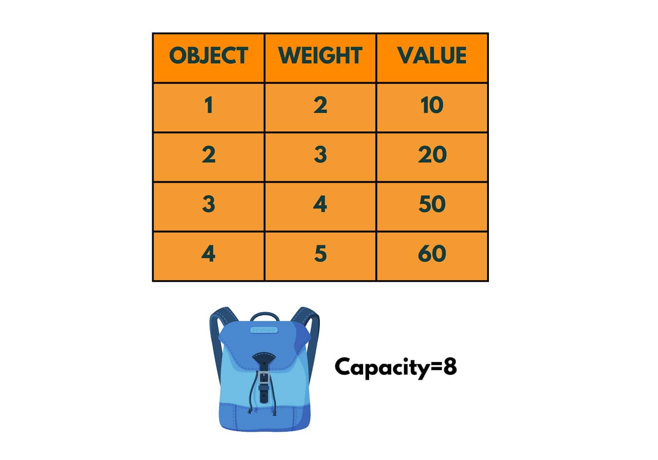
The problem requires us to fill the knapsack with these objects. Can we add all the objects to the knapsack? No, since the capacity of the knapsack is 8 while the total weight of the objects given is 14.
Hence, all the objects cannot be added to this knapsack, we need to carry only a few objects such that the total value of the objects is maximized. We need to give the solution in the form of a set x to trace whether item i is included in the knapsack (marked as 1) or not included (marked as 0).
Further, we'll explore how to solve this example using dynamic programming and the greedy algorithm.
Knapsack Problem Using Dynamic Programming
Before we start exploring how to solve the knapsack problem using dynamic programming, let us first understand what dynamic programming exactly is.
What is Dynamic Programming?
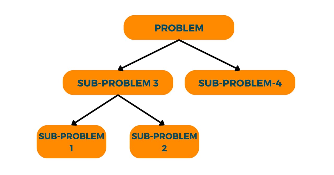
Dynamic programming is a technique for solving complex problems by breaking them down into smaller, more manageable subproblems and solving each subproblem only once, saving the results and reusing them as needed. It is a bottom-up approach that starts with solving the smallest subproblems and builds up to solve the larger ones.
The key idea behind dynamic programming is to avoid redundant calculations by storing the results of subproblems and using them to solve larger problems. This allows for efficient and fast computation, as many calculations are reused instead of being recalculated.
Dynamic programming is commonly used in computer science and other fields to solve optimization problems, such as the knapsack problem, shortest path problem, and maximum subarray problem, among others. It can also be applied to other types of problems, such as string matching, bioinformatics, and game theory.
Overall, dynamic programming is a powerful and versatile technique that allows for efficient and effective problem-solving in a wide range of applications.
maximize: ∑(i=1 to N) v(i)x(i) i.e. sum of their values needs to be maximized
subject to: ∑(i=1 to N) w(i)x(i) <= W i.e. sum of their weight should be less than or equal to the capacity of the knapsack.
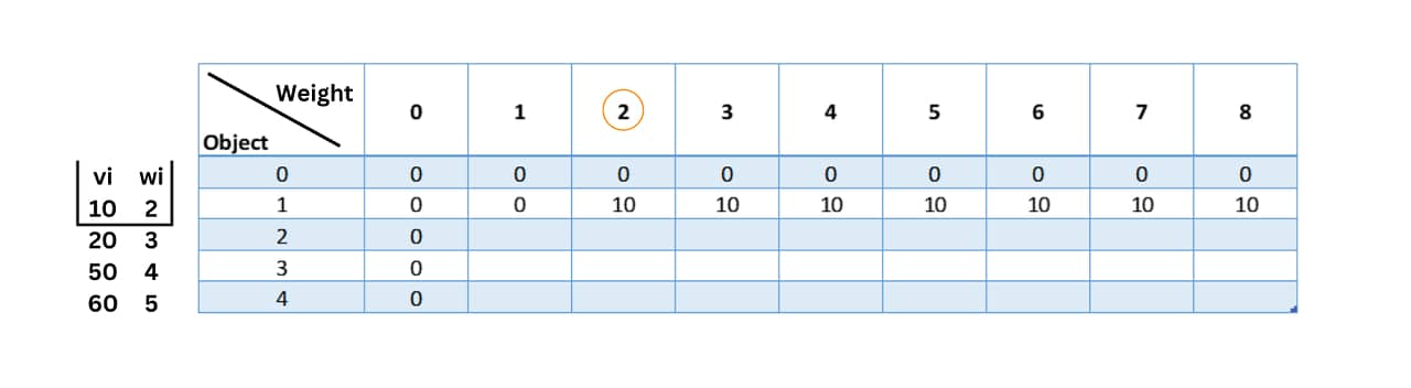
To solve this problem using the 0/1 knapsack algorithm, you can start by creating a table with one row for each item and one column for each possible weight from 0 to the knapsack capacity (8 in this case):
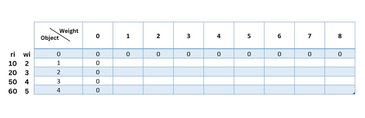
The cell in the row i and column j represents the maximum value that can be obtained using items 1 to i and a knapsack with a capacity j. The first row represents the case when there are no items, so the maximum value is always 0. The first column represents the case when the knapsack has no capacity, so the maximum value is always 0. vi and wi represent the values and weights of the specific objects.
Now, we start filling the table. We consider object 1 and ignore all other objects. We note that the weight of the first object is 2. The corresponding value is 10, so we fill the value '10' in table[1][2].
For the rest of the row, the capacity of the bag keeps increasing but since we are considering only one object i.e. object 1, we have nothing more to fill in the bag at that instance so we fill the same value throughout the row i.e. table[i][j]= table[i][j-1].
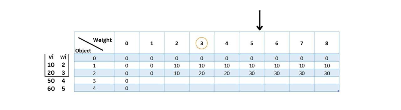
Let's fill the 2nd and the 3rd row in the same way with logic and then deduce the formula.
For the third row, when we consider the 2nd object, we should also include the first object. Let's look at the 2nd object. The weight of the second object is 3, hence, it can be where the weight of the bag is 3. Hence we fill table[2][3] with 20 which is the value of the bag.
For the left side of the column, we fill in the value from the previous row of the column i.e. table[i][j] will be equal to table[i-1][j].
Now, for the right side of the column, as I had mentioned earlier when we consider object 2 we also need to consider object 1. The total weight of the bag when we consider both objects is 5 and the total value will be 30. So for the weight column 5 we fill in 3 i.e. table[2][5]=30. Now, all the values after column 5 for object 2 will be 30 since in that instance the maximum value it holds is 30.
For the fourth row, we fill in the value for object 3 with weight 4 as 50 in table[3][4]. The left side of the table is filled with values from table[i-1][j]. We know that when we need to consider objects 1,2 and 3 while filling in the third row.
So when we consider objects 1 and 3 the total weight is 6 with the total value of the knapsack being 60.Further, when we consider objects 2 and 3 the total weight is 70 with the total value of the knapsack being 70. When we include all 3 the total weight is 10. Since the capacity of the knapsack is only 8 we cannot include all 3.
For the remaining vacant spaces, we fill them with the maximum value of the bag at the previous instance.
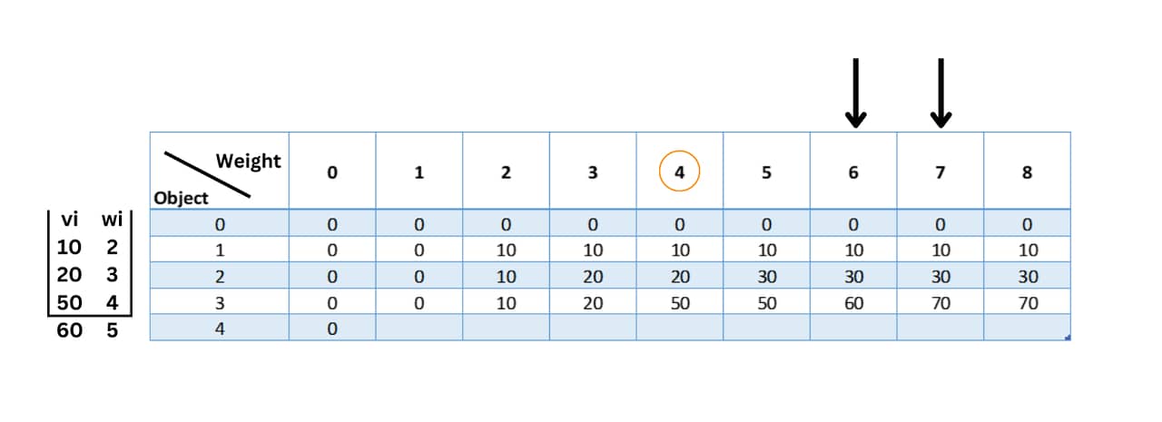
table[i][j] = max(table[i-1][j], values[i-1] + table[i-1][j-weights[i-1]])
table[4][2] = max(table[3][2], 60 + table[3][-3]) = max(10, undefined) = 10
table[4][3] = max(table[3][3], 60 + table[3][-2]) = max(20, undefined) = 20
table[4][4] = max(table[3][4], 60 + table[3][-1]) = max(50, undefined) = 50
table[4][5] = max(table[3][5], 60 + table[3][0]) = max(50, 60 + 0) = 60
table[4][6] = max(table[3][6], 60 + table[3][1]) = max(60, 60 + 0) = 60
table[4][7] = max(table[3][7], 60 + table[3][2]) = max(70, 60 + 10) = 70
table[4][6] = max(table[3][8], 60 + table[3][3]) = max(70, 70 + 10) = 80
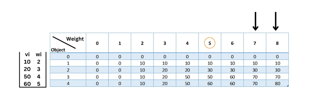
To determine which items should be included in the knapsack to obtain the maximum value, you can move vertically upward then trace back through the table from the last cell to the first cell, following the path with the values that don't originate from the top.
In this case, the path is (4,8) -> (2,3) -> (0,0). The value 80 doesn't come from the top which means this row is included. Similarly, the value 20 doesn't come from the top which means that row needs to be included.
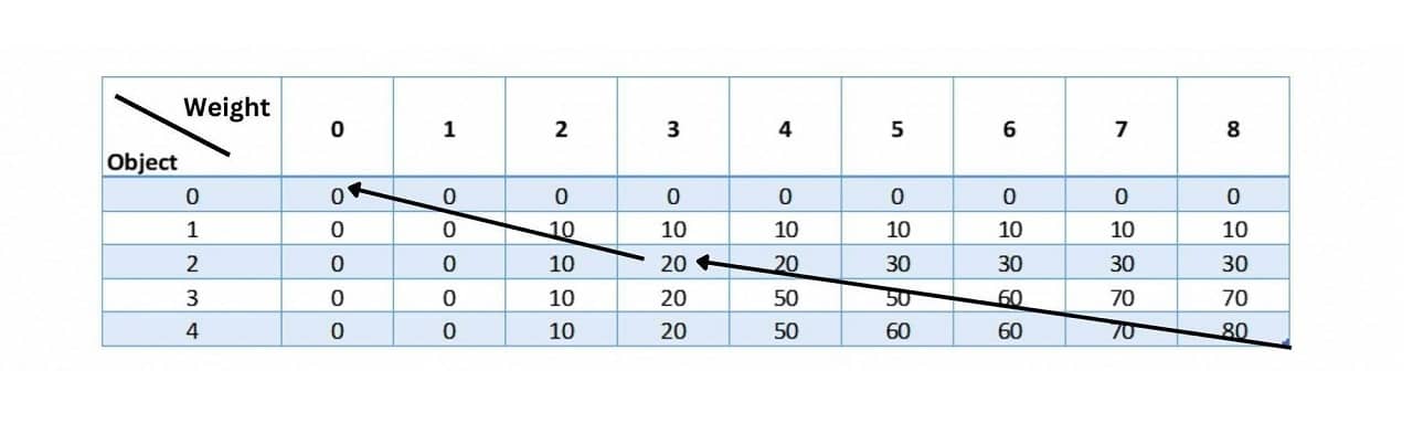
This path indicates that objects 4 and 2 should be included in the knapsack to obtain the maximum value of 80, without exceeding the weight capacity. Here is the C++ code:
#include <bits/stdc++.h>

using namespace std;

int knapsack(int capacity, vector<int>& wt, vector<int>& val, int n) {
    vector<vector<int>> dp(n + 1, vector<int>(capacity + 1, 0));

    for(int i = 1; i <= n; i++) {
        for(int j = 1; j <= capacity; j++) {
            if(wt[i - 1] > j) {
                dp[i][j] = dp[i - 1][j];
            }
            else {
                dp[i][j] = max(dp[i - 1][j], val[i - 1] + dp[i - 1][j - wt[i - 1]]);
            }
        }
    }

    return dp[n][capacity];
}

int main() {
    int capacity = 8; // maximum weight capacity of the knapsack
    vector<int> wt = {2, 3, 4, 5}; // weights of the items
    vector<int> val = {10, 20, 50, 60}; // values of the items
    int n = wt.size(); // number of items

    int maxVal = knapsack(capacity, wt, val, n);

    cout << "Maximum value that can be obtained: " << maxVal << endl;
}
Output:
Maximum value that can be obtained: 80
Time Complexity: O(N*W), where N is the total number of items and W is the capacity
Space Complexity: O(N*W), where N is the total number of items and W is the capacity
dp to store the maximum value that can be obtained for each combination of items and weight. We start with an empty knapsack and gradually add items one by one, considering both the case when we include the current item and when we do not include it.dp[n][capacity] represents the maximum value that can be obtained using all the items and a knapsack of capacity 8.def knapsack(capacity, wt, val, n): dp = [[0 for x in range(capacity+1)] for x in range(n+1)] for i in range(1, n+1): for j in range(1, capacity+1): if wt[i-1] > j: dp[i][j] = dp[i-1][j] else: dp[i][j] = max(dp[i-1][j], val[i-1] + dp[i-1][j-wt[i-1]]) return dp[n][capacity] capacity = 8 # maximum weight capacity of the knapsack wt = [2, 4, 4, 5] # weights of the items val = [10, 20, 50, 60] # values of the items n = len(wt) # number of items maxVal = knapsack(capacity, wt, val, n) print("Maximum value that can be obtained:", maxVal)
Maximum value that can be obtained: 80
Time Complexity: O(N*W), where N is the total number of items and W is the capacity
Space Complexity: O(N*W), where N is the total number of items and W is the capacity
0/1 Knapsack Problem using the Greedy Method
The 0/1 Knapsack problem is a classic optimization problem where we have a set of items, each with a weight and a value, and a knapsack with a maximum weight capacity. The goal is to choose a subset of items that fit into the knapsack and maximize the total value of the chosen items.
A greedy algorithm is an algorithmic paradigm that follows the problem-solving heuristic of making the locally optimal choice at each stage with the hope of finding a global optimum. However, the 0/1 Knapsack problem is not well-suited for a greedy approach, as choosing the items with the highest value-to-weight ratio at each step does not always lead to the optimal solution.
Here's an example to illustrate this:
Consider the following items:
- object 1: weight = 2, value = 10
- object 2: weight = 3, value = 20
- object 3: weight = 4, value = 50
- object 4: weight = 5, value = 60
And a knapsack with a capacity of 8.
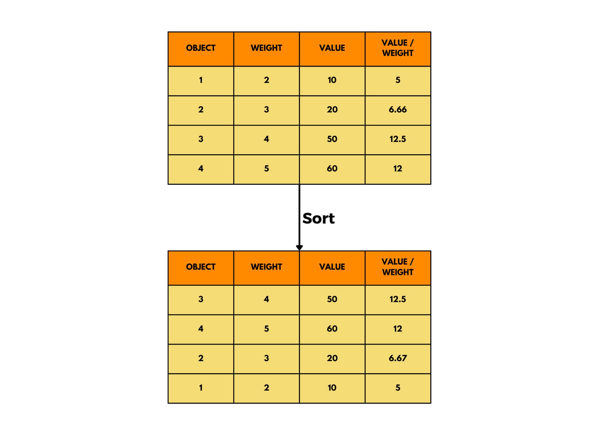
If we were to use a greedy algorithm to solve this problem, we would sort the items by the value-to-weight ratio in descending order as shown in the figure above, and then start adding the items one by one until the knapsack is full. The first item you would add will be the one with a value/weight ratio of 12.5 .i.e object 4 and then object 3 Using this approach, we would choose items 4 and 3, with a total value of 110. This is the wrong solution
However, the optimal solution would be to choose items 2 and 4, with a total value of 80. This can be seen by trying all possible combinations of items and selecting the one with the highest value that fits within the knapsack capacity using dynamic programming as seen above.
Therefore, a greedy algorithm is not always the best approach for the 0/1 Knapsack problem, and more advanced optimization techniques such as dynamic programming or branch-and-bound are usually needed to find the optimal solution.
Conclusion
Overall, the 0-1 Knapsack Problem is a fascinating challenge for computer scientists and mathematicians. Its applications span across industries, from finance and manufacturing to logistics and beyond, making it a perennial subject of interest and study.