Monte Carlo Simulations in R (with Examples)

Let's understand how to implement Monte Carlo Simulations in R.

What are Monte Carlo Simulations?

Generally, if you want to gain insights about a particular situation, you collect relevant data and analyze it. However, there are many cases where collecting real-time data is simply not feasible.

Also, if the situation has a lot of unpredictable factors, it can be difficult to collect enough data to reflect all this complexity. We may also want to explore hypothetical situations sometimes. This is why we need Monte Carlo simulations. Let’s understand in depth about it.

Monte Carlo simulation is a method in R for analyzing situations with uncertainty by mimicking them through repeated random sampling.

If you have a complex problem with many factors and unknown outcomes, instead of trying to solve it directly, you break it down into smaller parts and assign probabilities to different possibilities for each part.

Then, R lets you create thousands of virtual scenarios by randomly choosing values based on these probabilities. By analyzing the results of these scenarios, you gain insights into the overall outcome.

It’s not a perfect prediction, but it is valuable for informed decision-making. It makes the whole analysis process much less computationally expensive. This method is particularly useful when dealing with uncertainty, exploring "what-ifs", understanding complex systems, or when real data is not available or feasible.

Monte Carlo simulations in R can be applied to any problem involving uncertainty or randomness, including option pricing in finance, reliability analysis in engineering, clinical trial simulations in healthcare, and portfolio optimization. 

Understanding Monte Carlo Simulations

Monte Carlo is not a specific function in R, but rather an approach to problem-solving. Some important concepts in this technique are:

1) Random Sampling

This is the process of randomly picking elements to create samples. In the case of Monte Carlo simulations, there is no pre-existing population to draw samples from. So we use alternative methods:

1. Probability Distributions: Identify the probability distribution for the variable you're simulating. For example, a coin flip simulation follows the Bernoulli distribution with p = 0.5. Now, use built-in R functions to generate samples using this probability distribution. Some available functions are rbinom (Binomial), rnorm (Normal), and runif (Uniform).
2. Theoretical Models: If you have theoretical knowledge about the system or process you're simulating, develop or use an existing model to generate samples. This could involve solving equations, iterating through steps, or using specialized software.
3. Markov Chain Monte Carlo (MCMC): This is an advanced technique that creates a chain of samples where each new sample depends on the previous one, gradually covering the target distribution. Packages like mcmcpack and rjags in R support MCMC simulations.

2) Variance Reduction

Variance reduction techniques minimize the randomness and noise in Monte Carlo simulations, leading to more accurate results with less computational cost. There are various techniques available:

1. Antithetic sampling: This method pairs simulations with opposite values to cancel out some variation.
2. Control variates: This method uses known information to adjust simulations and reduce their randomness.
3. Stratified sampling: Dividing the simulated population into groups and drawing samples from each ensures a more balanced representation.
4. Importance sampling: This focuses on areas of the simulated population that contribute more to the outcome by adding weights, making simulations more efficient.

3) Parameter Estimation

This is to find the values of unknown parameters that best explain the behaviour of your simulated system. Here are some common approaches to parameter estimation in Monte Carlo simulations:

1. Maximum Likelihood Estimation (MLE): This is similar to making an educated guess. First, we guess different values of the parameters, then we run the simulations on each guess. Those that give results that look the most like the original are selected. The mle() function is used for this.
2. Bayesian Inference: This more advanced approach considers uncertainty in parameter values by treating them as probability distributions themselves. It uses information from both the data and prior knowledge (if available) to estimate the posterior distribution of parameters. Packages like mcmcpack and rjags can be used for this.
3. Method of Moments: This simpler method matches the moments (e.g., mean, variance) of your simulated data to the moments of the real-world data.
4. Genetic Algorithms: This method allows various guesses to compete. It selects and combines potential parameter sets based on how well they fit the data. It finds a population of good parameter sets, unlike MLE.  Packages like GA and rgenalg can be used for this.

Implementing Monte Carlo Simulations in R

So basically, this methodology involves the following steps:

1. Identifying variables, their interactions, and relevant values and probabilities.
2. Using R functions to generate random values based on your defined probabilities.
3. Employing various R functionalities for calculations, visualizations, and statistical tests.

Let’s look at this example where you want to find out the travelling time. You already know the average speed and distance, but consider potential delays due to traffic, weather, and detours (parameters). Here is how you implement this technique in R:

a) Define Variables

# Distance of the trip (in km)
distance <- 500

# Average travel speed (km/h)
speed <- 80

# Probabilities of different delay scenarios
p_traffic_delay <- 0.3          # 30% chance of traffic delay
delay_traffic <- 30             # Additional travel time due to traffic (minutes)

p_weather_delay <- 0.2      # 20% chance of weather delay
delay_weather <- 15         # Additional travel time due to weather (minutes)

p_detour <- 0.1                # 10% chance of detour
distance_detour <- 50       # Additional distance due to detour (km)

b) Simulate Scenarios

# Number of simulations
n_simulations <- 1000

# Generate random numbers for each delay scenario (Binomial Distributions)
traffic_delay <- rbinom(n_simulations, 1, p_traffic_delay) * delay_traffic
weather_delay <- rbinom(n_simulations, 1, p_weather_delay) * delay_weather
detour_distance <- rbinom(n_simulations, 1, p_detour) * distance_detour

# Calculate the total travel time for each simulation
travel_time <- distance / speed + (traffic_delay + weather_delay) / 60 +
  detour_distance / speed

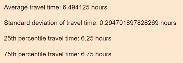
c) Analyze Results

# Average travel time
average_time <- mean(travel_time)
print(paste0("Average travel time: ", average_time, " hours"))

# Spread of travel times (e.g., standard deviation)
sd_time <- sd(travel_time)
print(paste0("Standard deviation of travel time: ", sd_time, " hours"))

# Calculate quantiles
quantile_time <- quantile(travel_time, c(0.25, 0.75))
# Print each quantile separately
print(paste0("25th percentile travel time: ", quantile_time[1], " hours"))
print(paste0("75th percentile travel time: ", quantile_time[2], " hours"))

Output:

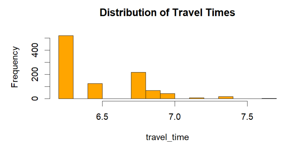
d) Visualize Findings

# Histogram of simulated travel times
hist(travel_time, main = "Distribution of Travel Times", col = "orange")

Output:

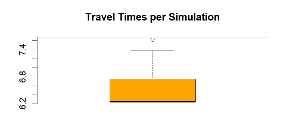
# Boxplot of travel times to see potential outliers
boxplot(travel_time, main = "Travel Times per Simulation", col = "orange")

Output:

Disadvantages of Monte Carlo Simulations

While powerful, Monte Carlo simulations (MCS) still have some limitations:

• It can be computationally expensive when there are too many parameters.
• It faces convergence challenges, that is, ensuring your simulation produces accurate results requires careful design and diagnostics to avoid getting stuck on misleading outcomes.
• It is not for deterministic problems. If you have an analytical solution to your problem, directly calculating the answer might be faster and more accurate.

Conclusion

Now here is how Monte Carlo Simulations are implemented in R. In conclusion, consider MCS when your problem involves complexity, randomness, incomplete data, or a need for statistical insights and sensitivity analysis. Just be mindful of its limitations.