
Random number generation is a crucial element of statistical analysis and simulation in R. A key player in generating random numbers in R is the rnorm() function, tailored for creating random numbers adhering to a normal distribution. This article will dive into the rnorm() function, explore its parameters and use cases, and understand how it contributes to the broader concept of random number generation in R.
Random Number Generation in R
Before we dive into the specifics of the rnorm() function, let's briefly discuss the importance of random number generation in statistical analysis and simulation. Many statistical techniques and machine learning algorithms rely on randomness, and the ability to generate random numbers is crucial for these applications.
R provides several functions for random number generation, catering to different distributions and requirements. The rnorm() function, in particular, is used for generating random numbers from a normal distribution. The normal distribution, often referred to as the Gaussian distribution, is a continuous probability distribution characterized by its bell-shaped curve.
What is the rnorm() Function?
The rnorm() function in R is relatively straightforward, yet powerful. Its basic syntax is as follows.
rnorm(n, mean = 0, sd = 1)
Here, 'n' signifies the number of random values to generate, 'mean' denotes the mean of the distribution, and 'sd' represents the standard deviation. By default, if 'mean' and 'sd' are not specified, the function generates random numbers from the standard normal distribution (mean = 0, sd = 1).
Let's explore each parameter in more detail.
n (Number of Random Values): This parameter specifies the number of random values to generate. It can be a single positive integer or a vector of integers. If n is a vector, the function will generate a random sample of size equal to the length of n.
mean (Mean of the Distribution): The mean of the normal distribution determines the center of the distribution. By default, it is set to 0. If a different mean is desired, you can specify it using the mean parameter.
sd (Standard Deviation): The standard deviation of the normal distribution controls the spread of the distribution. The default value is 1. If you want the distribution to have a different standard deviation, you can provide the desired value using the sd parameter.
Generating Random Numbers with Default Parameters
To get started, let's generate a simple random sample using the default parameters of the rnorm() function. We'll generate 100 random numbers from the standard normal distribution. Let's look at its code.
random_numbers <- rnorm(100)
In this example, random_numbers will be a numeric vector containing 100 random values drawn from the standard normal distribution.
Visualizing the Random Numbers
Visualizing the generated random numbers can provide insights into their distribution. We can use a histogram to observe the shape of the distribution. The following R code generates a histogram for the random sample we just created.
hist(random_numbers, main = "Histogram of Random Numbers", xlab = "Value", col = "lightblue", border = "black")
Plot:
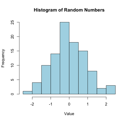
This code produces a histogram using the generated random numbers. The main parameter sets the title of the plot, and xlab specifies the label for the x-axis. The col and border parameters determine the color of the bars and their borders, respectively.
Customizing the Distribution with Mean and Standard Deviation
Although rnorm() typically generates random numbers from the standard normal distribution by default, you can tailor the distribution by specifying the mean and standard deviation. Let's create a random sample with a mean of 5 and a standard deviation of 2.
custom_numbers <- rnorm(100, mean = 5, sd = 2)
In this example, custom_numbers will be a numeric vector containing 100 random values drawn from a normal distribution with a mean of 5 and a standard deviation of 2.
Visualizing the Custom Distribution
To visualize the custom distribution, we can create another histogram.
hist(custom_numbers, main = "Histogram of Custom Random Numbers", xlab = "Value", col = "lightgreen", border = "black")
Plot:
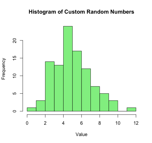
This histogram should show a distribution centered around the mean of 5, with a spread determined by the standard deviation of 2.
Generating Random Numbers for Simulation
The ability to generate random numbers is particularly useful for simulating scenarios and conducting statistical experiments. Let's consider a simple example where we simulate the rolling of a fair six-sided die. The outcomes of a fair die roll can be modeled using the rnorm() function by treating each face of the die as a category.
die_outcomes <- rnorm(100, mean = 3.5, sd = 1.7)
die_outcomes <- round(die_outcomes)
In this example, die_outcomes will be a numeric vector representing the simulated outcomes of rolling a fair six-sided die 100 times. The round() function is used to round the generated numbers to the nearest integer, ensuring that the outcomes correspond to the faces of the die.
Visualizing the Simulated Die Rolls
To visualize the simulated die rolls, we can create a bar plot to display the frequency of each outcome.
barplot(table(die_outcomes), main = "Simulated Die Rolls", xlab = "Die Face", ylab = "Frequency", col = "skyblue")
Plot:
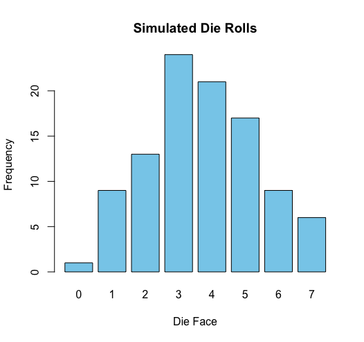
This code uses the table() function to calculate the frequency of each unique outcome in die_outcomes and then creates a bar plot to display the distribution of simulated die rolls.
Advanced Features of rnorm()
Let's now discuss some of the more advanced features in rnorm() which let us take the usage of randomness in our programs to the next level.
1. Seed for Reproducibility
In statistical analysis and simulation, reproducibility is often crucial. Setting a seed ensures that the same set of random numbers is generated every time the code is run. The set.seed() function in R is used for this purpose. Here's an example.
Code:
set.seed(123)

reproducible_numbers <- rnorm(100)

head(reproducible_numbers)
Output:
-0.56047565 -0.23017749 1.55870831 0.07050839 0.12928774 1.71506499
By setting the seed to a specific value (in this case, 123), the random numbers generated by rnorm() will be the same each time the code is executed. You can run the code and get the same output.
2. Generating Correlated Random Variables
The rnorm() function is versatile and can generate correlated random variables by specifying a covariance matrix. For this purpose, the mvrnorm() function from the MASS package can be particularly handy. Here's a brief example.
Code:
install.packages("MASS")
library(MASS)

set.seed(123)

cov_matrix <- matrix(c(1, 0.7, 0.7, 1), nrow = 2)

correlated_variables <- mvrnorm(n = 100, mu = c(0, 0), Sigma = cov_matrix)

head(correlated_variables)
Output:
           [,1]        [,2]
[1,] -0.2415937 -0.79187229
[2,] -0.3117038 -0.11272253
[3,]  1.5326014  1.34151471
[4,]  0.1996082 -0.06959715
[5,]  0.4877577 -0.24936288
[6,]  1.5986510  1.56377263
In this example, cov_matrix is a 2x2 matrix representing the covariance between two variables. The mvrnorm() function generates random variables with the specified covariance matrix.
Conclusion
In summary, the rnorm() function in R plays a crucial role in generating random numbers, especially from a normal distribution, making it essential for statistical analyses and simulations. This article explored its core parameters, showcasing its adaptability in shaping distributions through mean and standard deviation adjustments. Through practical examples, we demonstrated its usefulness in generating random samples, simulating scenarios, and modeling correlated variables. The guide also emphasized the importance of seed setting for reproducibility in research and analysis.