

Dimensionality reduction and data visualization are key concepts in data science. Principal Component Analysis (PCA) is a powerful statistical method that addresses both of these concepts. It works by transforming data from a high-dimensional space to a lower-dimensional one while preserving meaningful properties of the original data. This helps reveal patterns and insights, making PCA an important tool for exploring and interpreting data. In this article, we'll dive into the fundamentals of PCA and its implementation in the R programming language. We'll cover important concepts, the use of the prcomp function in R, the significance of eigenvalues, and how to interpret the PCA results.
Understanding Principal Component Analysis (PCA)
PCA is a technique widely employed in various fields such as finance, biology, natural sciences, and image analysis. PCA aims to simplify complex datasets by transforming them into a new coordinate system, where the axes are the principal components of the dataset. Principal components are linear combinations of the original variables and are arranged in descending order of importance. The first principal component captures the maximum variance in the data, with the next components explaining decreasing amounts of variance in order.
Implementation of PCA in R
R is a popular programming language for research-based statistical computing and graphical analysis. The prcomp function is a key player in this process. Let's walk through a basic example to illustrate the implementation of PCA in R.
Code:
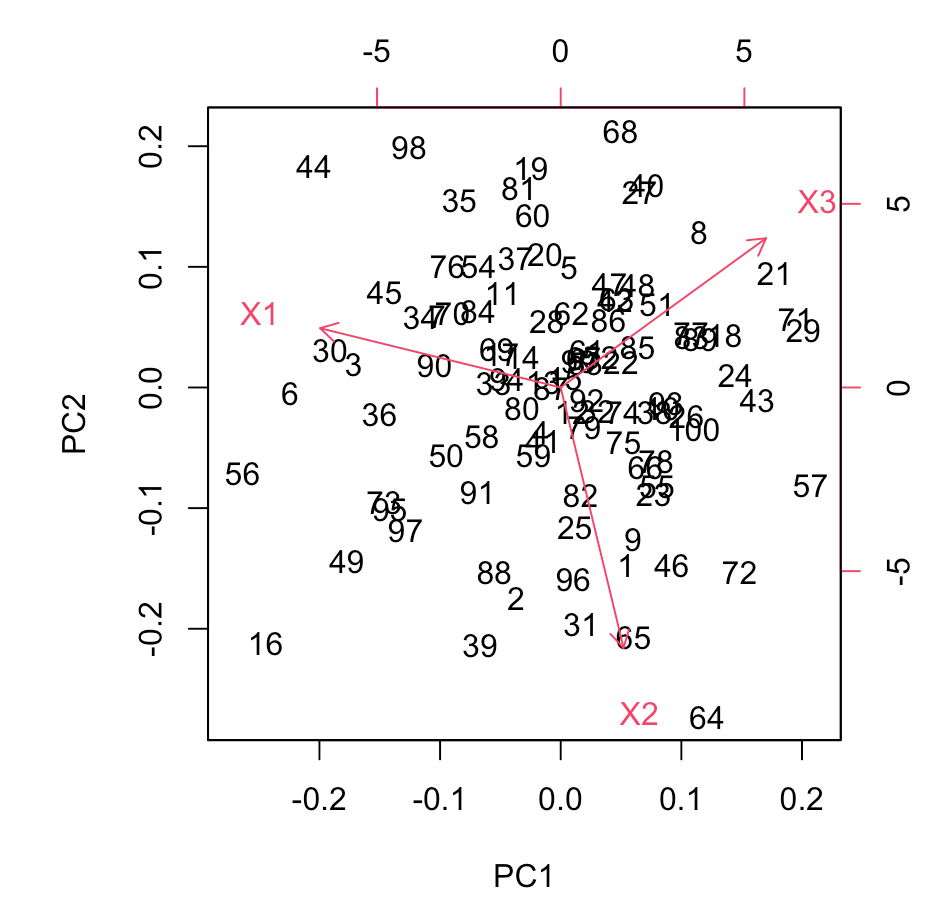
library(ggplot2)

set.seed(123)
data <- data.frame(
  X1 = rnorm(100),
  X2 = 2 * rnorm(100) + 3 * rnorm(100),
  X3 = 0.5 * rnorm(100) + 2 * rnorm(100)
)

scaled_data <- scale(data)

pca_result <- prcomp(scaled_data, center = TRUE, scale. = TRUE)

summary(pca_result)

screeplot(pca_result, type = "lines", main = "Scree Plot")

biplot(pca_result)
Output:
Importance of components:
                          PC1    PC2    PC3
Standard deviation     1.0973 1.0410 0.8439
Proportion of Variance 0.4014 0.3612 0.2374
Cumulative Proportion  0.4014 0.7626 1.0000
Scree Plot
In this example, we first generate a synthetic dataset with three variables (X1, X2, and X3). The data is then standardized using the scale function to ensure that variables are on a comparable scale. The prcomp function is applied to perform PCA, and the results are summarized.
A scree plot is generated to visualize the proportion of variance explained by each principal component, providing insights into the dataset's structure.
Eigenvalues in PCA
Eigen value is an important factor to be considered in PCA, as it represents the different variance captured by each principal components. The eigenvalues are extracted from the covariance matrix of the standardized data. The total sum of eigenvalues equals the total variance in the dataset.
Let's extend our previous R example to include the extraction and analysis of eigenvalues.
Code:
eigenvalues <- pca_result$sdev^2

variance_proportion <- eigenvalues / sum(eigenvalues)

eigenvalues_table <- data.frame(
  Principal_Component = 1:length(eigenvalues),
  Eigenvalue = eigenvalues,
  Variance_Proportion = variance_proportion
)

print("Eigenvalues and Variance Proportion:")
print(eigenvalues_table)
Output:
Eigenvalues and Variance Proportion:
  Principal_Component Eigenvalue Variance_Proportion
1                   1  1.2041240           0.4013747
2                   2  1.0836328           0.3612109
3                   3  0.7122433           0.2374144
We extract eigenvalues from the pca_result object and calculate the proportion of total variance explained by each principal component. The table provides a clear overview of the eigenvalues and their significance. Analysts often refer to a scree plot, as shown earlier, to visually assess the drop-off in eigenvalues, helping determine the number of principal components to retain.
PCA Interpretation in R
Interpreting the results of PCA involves a detailed analysis of loadings and their relationships to the original variables. Loadings represent the correlations between the original variables and the principal components, providing insights into how much each variable contributes to the identified patterns.
Code:
loadings <- pca_result$rotation

print("Loadings:")
print(loadings)
Output:
Loadings:
          PC1        PC2       PC3
X1 -0.7460842  0.1938464 0.6370102
X2  0.1949652 -0.8511566 0.4873613
X3  0.6366687  0.4878074 0.5972411
In this code, we extract the loadings from the pca_result object, which represent the correlations between the original variables and the principal components. The resulting table provides a representation of these loadings. You can use this information to identify patterns and relationships between variables.
Here in our case, PC1, PC2, and PC3 represent the different principal components. The number shows how positively or negatively they are affecting the variables. -0.8511566 shows a strong negative impact, while 0.6370102 represents a strong positive impact.
The direction of the loading, whether positive or negative, denotes the nature of the relationship. A positive loading implies that an increase in the variable corresponds to an increase in the principal component's score, while a negative loading suggests the opposite.
Conclusion
Principal Component Analysis (PCA) is a valuable technique for discovering patterns and simplifying complex datasets. By exploring eigenvalues and loadings, analysts can extract valuable insights into the structure and relationships within their data, easily achieved using the prcomp function. Visual aids like the scree plot further assist in interpreting PCA results. PCA is a versatile method that can be applied to various domains. Using the R programming language, you can easily use this method to interpret and explore data.