
Logistic regression is a powerful tool for analyzing and predicting binary outcomes in the large world of statistical modelling. Understanding logistic regression in the R programming language is an important skill for anyone interested in data science or doing research. In this article, we'll learn about doing logistic regression analysis in R, with a focus on the glm function and how it's used in binary logistic regression.
Basics of Logistic Regression
Logistic regression is a statistical method used when the dependent variable is binary, meaning it has only two possible outcomes. These outcomes are often coded as 0 and 1, representing, for instance, failure and success, presence and absence, or yes and no. The fundamental idea behind logistic regression is to model the probability that a given instance belongs to a particular category.
R's glm (generalized linear model) function is essential for fitting logistic regression models. It has the following syntax:
model <- glm(formula, data = dataset, family = "binomial")
Here, "formula" specifies the relationship between the predictor variables and the response variable, "data" refers to the dataset, and "family" is set to "binomial" to indicate logistic regression.
Understanding the Formula
The formula in the glm function is crucial in defining the relationship between the predictor variables and the response variable. The formula follows the pattern:
response_variable ~ predictor_variable1 + predictor_variable2 + ... + predictor_variableN
For example, if we are examining the relationship between a student's exam success (1 for success, 0 for failure) and the number of hours spent studying and the type of study materials used, the formula might look like:
success ~ hours_studied + type_of_material
Let’s start the process by first creating the data for analysis.
Data Preparation
It is important to properly prepare the data before getting into logistic regression analysis. We need to make sure that the dependent variable is coded as a binary outcome (0 or 1) and that the feature variables are properly typed. Convert categorical variables to factors using the 'factor' function ensuring that R recognizes them as such during the model training process.
Installing Packages and loading data
Before we jump into code, let's ensure that the necessary packages are installed. We'll need the "titanic" package for the dataset, along with "dplyr" for data manipulation and "broom" for tidying up model outputs.
# Install and load necessary packages
install.packages("titanic")
install.packages("dplyr")
install.packages("broom")

library(titanic)
library(dplyr)
library(broom)
Now that our packages are installed, let's load the Titanic dataset and look at its structure using the "str" function.
# Load the Titanic dataset
data("titanic_train")
titanic_data <- titanic_train

# Explore the structure of the dataset
str(titanic_data)
Output:
'data.frame':	891 obs. of  12 variables:
 $ PassengerId: int  1 2 3 4 5 6 7 8 9 10 ...
 $ Survived   : int  0 1 1 1 0 0 0 0 1 1 ...
 $ Pclass     : int  3 1 3 1 3 3 1 3 3 2 ...
 $ Name       : chr  "Braund, Mr. Owen Harris" "Cumings, Mrs. John Bradley (Florence Briggs Thayer)" "Heikkinen, Miss. Laina" "Futrelle, Mrs. Jacques Heath (Lily May Peel)" ...
 $ Sex        : chr  "male" "female" "female" "female" ...
 $ Age        : num  22 38 26 35 35 NA 54 2 27 14 ...
 $ SibSp      : int  1 1 0 1 0 0 0 3 0 1 ...
 $ Parch      : int  0 0 0 0 0 0 0 1 2 0 ...
 $ Ticket     : chr  "A/5 21171" "PC 17599" "STON/O2. 3101282" "113803" ...
 $ Fare       : num  7.25 71.28 7.92 53.1 8.05 ...
 $ Cabin      : chr  "" "C85" "" "C123" ...
 $ Embarked   : chr  "S" "C" "S" "S" ...
This dataset contains various details about passengers, but for our logistic regression model, we'll focus on three key elements: survival status ("Survived"), passenger class ("Pclass"), and age ("Age").
Data Preprocessing
Next step is to preprocess the data ensuring it is perfect for the smooth conduct of the analysis. We'll take care of any missing values, pick the appropriate columns, and factorize the passenger class.
# Data preprocessing
# Select relevant columns: Survived, Pclass, Age
selected_columns <- c("Survived", "Pclass", "Age")
titanic_data <- select(titanic_data, all_of(selected_columns))

# Remove rows with missing values
titanic_data <- na.omit(titanic_data)

# Convert Pclass to a factor
titanic_data$Pclass <- as.factor(titanic_data$Pclass)

# Display the first few rows of the preprocessed data
head(titanic_data)
Output:
  Survived Pclass Age
1        0      3  22
2        1      1  38
3        1      3  26
4        1      1  35
5        0      3  35
7        0      1  54
Our dataset has been carefully selected to only contain the variables that are necessary for our analysis. For proper modelling, the passenger class has been turned into a factor and rows containing missing values have been removed.
Fitting a Logistic Regression Model
Using the "glm" function, we'll model the probability of survival based on passenger class and age.
# Fitting a logistic regression model
logreg_model <- glm(Survived ~ Pclass + Age, data = titanic_data, family = "binomial")

# View the summary of the model
summary(logreg_model)
Output:
Call:
glm(formula = Survived ~ Pclass + Age, family = "binomial", data = titanic_data)

Deviance Residuals:
    Min       1Q   Median       3Q      Max
-2.1524  -0.8466  -0.6083   1.0031   2.3929

Coefficients:
             Estimate Std. Error z value Pr(>|z|)
(Intercept)  2.296012   0.317629   7.229 4.88e-13 ***
Pclass2     -1.137533   0.237578  -4.788 1.68e-06 ***
Pclass3     -2.469561   0.240182 -10.282  < 2e-16 ***
Age         -0.041755   0.006736  -6.198 5.70e-10 ***
---
Signif. codes:  0 ‘***’ 0.001 ‘**’ 0.01 ‘*’ 0.05 ‘.’ 0.1 ‘ ’ 1

(Dispersion parameter for binomial family taken to be 1)

    Null deviance: 964.52  on 713  degrees of freedom
Residual deviance: 827.16  on 710  degrees of freedom
AIC: 835.16

Number of Fisher Scoring iterations: 4
Here we are fitting a logistic regression model, with survival as the response variable and passenger class and age as predictors. The summary provided us with necessary information such as the coefficients, standard errors, z-values, and p-values. Interpreting coefficients involves understanding how a one-unit change in a feature variable affects the target variable's log-odds. For categorical variables, the interpretation involves comparing one category to a reference category.
Assessing Model Performance
Evaluating the performance of the logistic regression model is crucial to ensure its reliability and generalizability. Common techniques are examining the confusion matrix, calculating accuracy, precision, recall, and the area under the receiver operating characteristic (ROC) curve.
Let’s check out the code for them.
# Assessing model performance
predicted_values <- predict(logreg_model, newdata = titanic_data, type = "response")
predicted_classes <- ifelse(predicted_values > 0.5, 1, 0)

# Confusion matrix
conf_matrix <- table(observed = titanic_data$Survived, predicted = predicted_classes)
conf_matrix

# ROC curve
library(pROC)
roc_curve <- roc(titanic_data$Survived, predicted_values)
plot(roc_curve, main = "ROC Curve", col = "blue", lwd = 2)
Confusion Matrix
        predicted
observed   0   1
       0 344  80
       1 138 152
ROC Curve Plot
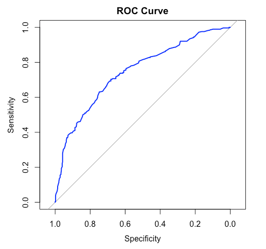
ROC curves and confusion matrix gives us an insight to how our models perform on the testing data - the new and unseen data. This provides us with a general idea about the model's accuracy and performance. From the confusion matrix we also can calculate other important details such as the precision and recall of the model which gives beneficial insights in research and development fields.
Conclusion
Logistic regression in R is an efficient and powerful way to model binary outcomes. You can learn a lot about the relationships in your data by comprehending the fundamentals of logistic regression, data preparation, model fitting, coefficient interpretation, and model evaluation. It opens up a lots of opportunities in statistics driven decision making as a data scientist.