.png)
Broadly, there are 3 paradigms of Machine Learning: Supervised Learning, Unsupervised Learning, and Reinforcement Learning. In Supervised Learning, a Machine Learning Model is trained using a learning algorithm that takes both the features and target (to be predicted) into account whereas, in Unsupervised Learning, a Machine Learning Model (mostly Pattern Recognition) is trained using a learning algorithm that takes only the features into account. Reinforcement Learning refers to Active Learning which is out of the scope of this discussion. So, intuitively Supervised Learning should be more successful than Unsupervised Learning as it is trained by taking both the features and target into account unlike Unsupervised Learning that only relies on features: pattern matching & recognition among them for mostly classification purposes.
What is K means clustering?
K means clustering is a learning algorithm following the Unsupervised Learning paradigm. It is based on the intuition of Pattern Recognition on n-dimensional feature-space geometry. In n-dimensional feature-space geometry, each and every data instance is visualized as a data-point in n dimensions in which the n dimensions are the n features.
K means clustering algorithm:
1. Randomly selecting k cluster centroids
2. Assigning all the data-points (except the k data-points that are k cluster centroids themselves) to the k clusters based on euclidean distance
3. Updating cluster centroids for each of the k clusters by taking the mean of the data points in each cluster across every dimension
4. Repeat steps 2 and 3 until cluster centroids change no more after step 3.
10 Steps to Build K means clustering in Python With Performance Analysis
1. Importing necessary libraries
# importing the necessary libraries
import warnings
warnings.filterwarnings('ignore')
import numpy as np
import pandas as pd
from sklearn.preprocessing import StandardScaler
from sklearn.decomposition import IncrementalPCA
from sklearn.cluster import KMeans
from sklearn import metrics
import matplotlib.pyplot as plt
2. Reading the Breast Cancer Wisconsin (Diagnostic) Dataset
# reading the Breast Cancer Wisconsin (Diagnostic) Data Set
df = pd.read_csv('data.csv')

# displaying top 5 instances of the dataset
print(df.head())
Corresponding Output
         id diagnosis  radius_mean  texture_mean  perimeter_mean  area_mean  \
0    842302         M        17.99         10.38          122.80     1001.0
1    842517         M        20.57         17.77          132.90     1326.0
2  84300903         M        19.69         21.25          130.00     1203.0
3  84348301         M        11.42         20.38           77.58      386.1
4  84358402         M        20.29         14.34          135.10     1297.0

   smoothness_mean  compactness_mean  concavity_mean  concave points_mean  \
0          0.11840           0.27760          0.3001              0.14710
1          0.08474           0.07864          0.0869              0.07017
2          0.10960           0.15990          0.1974              0.12790
3          0.14250           0.28390          0.2414              0.10520
4          0.10030           0.13280          0.1980              0.10430

   ...  texture_worst  perimeter_worst  area_worst  smoothness_worst  \
0  ...          17.33           184.60      2019.0            0.1622
1  ...          23.41           158.80      1956.0            0.1238
2  ...          25.53           152.50      1709.0            0.1444
3  ...          26.50            98.87       567.7            0.2098
4  ...          16.67           152.20      1575.0            0.1374

   compactness_worst  concavity_worst  concave points_worst  symmetry_worst  \
0             0.6656           0.7119                0.2654          0.4601
1             0.1866           0.2416                0.1860          0.2750
2             0.4245           0.4504                0.2430          0.3613
3             0.8663           0.6869                0.2575          0.6638
4             0.2050           0.4000                0.1625          0.2364

   fractal_dimension_worst  Unnamed: 32
0                  0.11890          NaN
1                  0.08902          NaN
2                  0.08758          NaN
3                  0.17300          NaN
4                  0.07678          NaN
3. Dropping unwanted columns, 'id' and 'Unnamed: 32' are dropped
# the unwanted columns, 'id' and 'Unnamed: 32' are dropped
df.drop(['id', 'Unnamed: 32'], axis = 1, inplace = True)
4. Label Encoding of the Target Variable
# label-encoding of the target label, 'diagnosis' such that B(Benign) -> 0 and M (Malignant) -> 1
df['diagnosis'] = df['diagnosis'].map({'B':0, 'M':1})
5. Creating the Feature Set and Target Label variables
# spliting into X (features) and y (target label)
X = df.iloc[:, 1:]
y = df['diagnosis']
6. Feature Scaling
# feature scaling
X_scaled = StandardScaler().fit_transform(X)
7. Principal Component Analysis (PCA) to reduce the dimensionality of the data into 2 dimensions
# Incremental Principal Component Analysis to select 2 features such that they explain as much variance as possible
pca = IncrementalPCA(n_components = 2)
X_pca = pca.fit_transform(X_scaled)
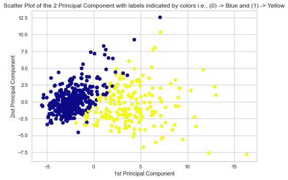
8. Scatter-Plot Visualization of the 2 Principal Components
# Scatter Plot of the 2 Principal Components with labels indicated by colors
plt.scatter(X_pca[:,0], X_pca[:,1], c = y, cmap = 'plasma')
plt.xlabel('1st Principal Component')
plt.ylabel('2nd Principal Component')
plt.title('Scatter Plot of the 2 Principal Component')
plt.show()
Corresponding Output
9. k means Clustering with 2 clusters signifying the 2 classes (Benign -> 0 and Malignant -> 1)
# k-Means Clustering with 2 clusters as there are 2 labels
model = KMeans(n_clusters = 2, random_state=1234).fit(X_pca)
y_cluster = model.predict(X_pca)
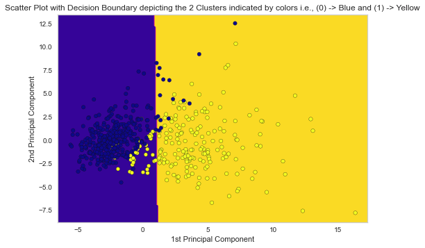
10. Performance Analysis of the k Means Clustering and Performance Visualization using Decision Boundary on Scatter-Plot
# Getting the Accuracy of the k-Means Clustering Model
print('Accuracy of the Model: ', metrics.accuracy_score(y, y_cluster))
print()

# Getting the Precision of the k-Means Clustering Model
print('Precision of the Model: ', metrics.precision_score(y, y_cluster))
print()

# Getting the Recall of the k-Means Clustering Model
print('Recall of the Model: ', metrics.recall_score(y, y_cluster))
print()

# Getting the F1-Score of the k-Means Clustering Model
print('F1-Score of the Model: ', metrics.f1_score(y, y_cluster))
print()
Corresponding Output
Accuracy of the Model:  0.9068541300527241

Precision of the Model:  0.9162303664921466

Recall of the Model:  0.8254716981132075

F1-Score of the Model:  0.8684863523573201
# plotting the decision boundary in the scatter plot of the 2 Principal Components with labels indicated by colors
x_min, x_max = X_pca[:, 0].min() - 1, X_pca[:, 0].max() + 1
y_min, y_max = X_pca[:, 1].min() - 1, X_pca[:, 1].max() + 1

xx, yy = np.meshgrid(np.arange(x_min, x_max, 0.1),
                     np.arange(y_min, y_max, 0.1))

Z = model.predict(np.c_[xx.ravel(), yy.ravel()])
Z = Z.reshape(xx.shape)

plt.contourf(xx, yy, Z, cmap = 'plasma')
plt.scatter(X_pca[:, 0], X_pca[:, 1], c = y, s = 30, edgecolor = 'k', cmap = 'plasma')
plt.xlabel('1st Principal Component')
plt.ylabel('2nd Principal Component')
plt.title('Scatter Plot with Decision Boundary depicting the 2 Clusters indicated by colors i.e., (0) -> Blue and (1) -> Yellow')
plt.show()
Corresponding Output
Applications of k means clustering
Some of the practical applications of k means clustering are as follows:
1. Market Segmentation where there is a database of customers and grouping them down to different market segments
2. Social Network Analysis
3. Cluster Computing Design in Data Centres
4. Astronomical Data Analysis to interpret galaxy formations
5. Document/Topic Clustering
Conclusion
From the Performance Analysis (Accuracy, Precision, Recall and F1-Score) and Visualization (Decision Boundary), the Unsupervised Learning Model, k Means Clustering in python performed really well even though no target label is taken into account in the Model Development process.


.png)