Creating Density Plot in R (with Examples)

Visualizing data is important because it helps to easily understand data, identify patterns, compare scenarios, and detect errors. It is also useful in communicating findings effectively and presenting the story of the data backed up by evidence. As they say, a picture is worth a thousand words. In this article, we will look at one such visualization: Density Plots in R.

What is a Density Plot in R?

A density plot is a graphical representation of the probability distribution of a continuous variable. But in simpler terms, it is a way to show how data is spread out along a range of values. It helps you see the shape of your data so that you can understand where the data is concentrated. Understanding this distribution is the first thing you need to do after importing your data.

Below are some important components of density plots that will help you understand the concept better.

1. Kernel Function: A kernel function is like a smooth and symmetric bump that you place on each data point. It is a way to emphasize that specific point.
2. Kernel Density Estimation (KDE): When you add up all these little bumps from every data point, you get a Kernel Density Estimation (KDE). It is like smoothing out all the bumps and creating a continuous curve that shows you how the data is spread out.
3. Bandwidth: It controls how much you want to smooth out these bumps while creating the curve from the kernels. So basically, it defines the smoothness of the curve. A low bandwidth can capture small details in the data but results in a noisy estimate. On the other hand, high bandwidth gives a general sense of the distribution but misses small details.

KDE is calculated using the following formula:

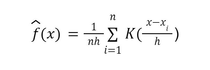
where:
n is the number of data points in the sample.
h is the bandwidth of the kernel.
xi represents each data point in the sample.
K() is the kernel function.

Types of Density Plots 

The following are the types of density plots:

1. Univariate Density Plot: This is used to estimate the probability density function of a single variable.
2. Multivariate Density Plot: This is used when you want to estimate the probability density function of multiple variables. It is generally suggested to not use more than 3 variables at once as it can become messy and confusing.

Creating Density Plots in R

Let’s check out the syntax of creating density plots in R:

ggplot(data, aes(x)) +
  geom_density(fill, color, alpha, size, linetype, kernel, adjust, trim, na.rm) +
  labs(x, y, title)

You need not use each of these parameters every time you want to create a density plot. Most of these are to customize the look and feel of your plot. Using these can also help to differentiate between multiple plots on the same graph. Here’s what each of these attributes do:

• data: Specifies the dataset.
• aes: Defines the aesthetic mappings by linking variables to plot aesthetics.
• x: Specifies the variable in the data that you want to visualize.
• fill: Fills the color of the density curve.
• color: Fills the border color of the density curve.
• alpha: Sets the transparency of the fill color. It is a numeric value between 0 (completely transparent) and 1 (completely opaque).
• size: Sets the line size of the density curve. It is a numeric value.
• linetype: Sets the line type of the density curve. It can be one among c("blank", "solid", "dashed", "dotted", "dotdash", "longdash", "twodash").
• kernel: Defines the kernel type for kernel density estimation. It can be one among c("gaussian", "rectangular", "triangular", "epanechnikov", "biweight", "cosine", "optcosine") depending on your data.
• adjust: Adjusts bandwidth for the kernel density estimate. It is a numerical value.
• trim: Defines whether to trim density estimates outside the data range. It is a boolean value.
• na.rm: Defines whether to remove NAs from the data before plotting. It is a boolean value.
• labs(x, y, title): Gives labels for the axes and the plot title.

Let’s check an example of the same:

# Load necessary library
library(ggplot2)

# Create a simple univariate density plot using the iris dataset
ggplot(data = iris, aes(x = Sepal.Length)) +
  geom_density(fill = "blue", color = "black", alpha = 0.5, size = 1, linetype = "solid", 
               kernel = "gaussian", adjust = 1, trim = FALSE, na.rm = FALSE) +
  labs(x = "Sepal Length (cm)", y = "Density", title = "Univariate Density Plot")

Output:

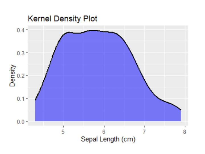
From this output, you can see that the sepal lengths of most fall in the range of 5 to 6.5 cm.

Similarly, we can create a bivariate density plot using the 'ggplot' library and the geom_density_2d function.

ggplot(data = iris, aes(x = Sepal.Length, y = Sepal.Width)) +
  geom_density_2d(fill=”blue”, color = "red", alpha = 0.7, size = 0.5) +
  labs(x = "Sepal Length (cm)", y = "Sepal Width (cm)", title = "Bivariate Density Plot")

Output:

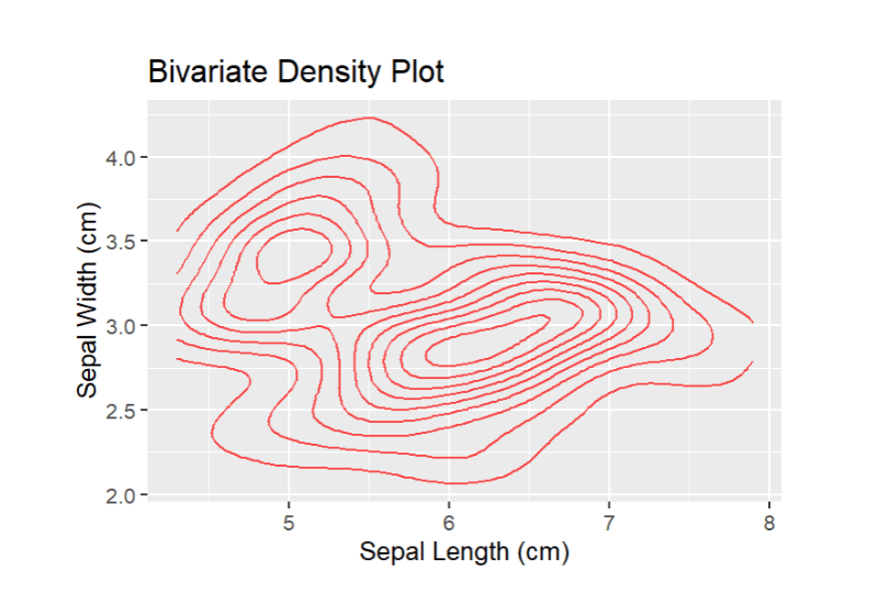
This pattern suggests that Sepal Length and Sepal Width don't exhibit a clear positive or negative linear relationship.

Enhancing Density Plots

This is used to provide a more accurate representation of the underlying data. Some ways to enhance density plots are:

1) Bandwidth Selection

Adjusting the bandwidth helps to find the right balance between capturing details and creating an understandable representation. Many bandwidth selection methods can be used for this purpose. 

The most common ones are:

• Scott's Rule: It automatically adjusts the smoothing based on how spread out or packed your data is.
• Silverman's Rule: It is similar to Scott’s but with a little extra smoothing.
• Cross-Validation: It involves testing different bandwidths and picking the one that gives the best balance between detail and smoothness.

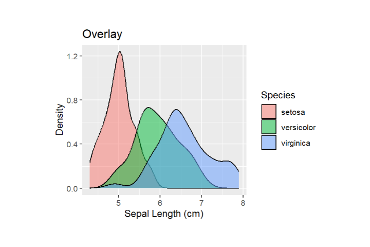
2) Multiple Curves in One Plot

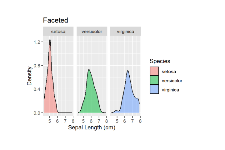
You can either overlay multiple plots on the same graph, or facet the plot to create separate panels for each category. This is useful for comparisons.

# Overlay Density Plots for Different Species in the Same Plot
ggplot(data = iris, aes(x = Sepal.Length, fill = Species)) +
  geom_density(alpha = 0.5) +
  labs(x = "Sepal Length (cm)", y = "Density", title = "Density Plots by Species")

# Facet the Plot for Separate Panels
ggplot(data = iris, aes(x = Sepal.Length, fill = Species)) +
  geom_density(alpha = 0.5) +
  facet_wrap(~Species) 

Output:

3) Color Mapping, Transparency and Contouring

Using color mapping to represent density levels can make your visualization clearer. The same thing can be done by adjusting transparency, which ensures that overlapping areas are darker. Similarly, contour lines can be added to highlight areas with specific density levels.

Conclusion

Overall, density plots in R are used to visualize the probability distribution of the given data to understand data spread and compare between groups. The key to an accurate density plot lies in the customization options. Choosing the right kernel function, bandwidth and aesthetics help you tell the story behind your data in a better way.