
The role of credit cards as a method of transaction has gained a lot of popularity over the years as the world aims to be a cashless society. However, it is also important to consider that credit card fraud is ranked as the most common kind of identity theft fraud. One of the principal tasks that can be done by machine learning algorithms is classification. Every credit card transaction results in the generation of some data that can be used by machine learning algorithms to develop a classifier. Using such a classifier in real-time can help detect fraudulent transactions almost immediately resulting in not only time being saved but also money. In this post, a random forest classifier will be implemented to predict whether a transaction is a valid transaction or a fraudulent one.
Importing the Libraries
Several libraries will be used for different purposes in this post. The pandas library will be used to load the data into a DataFrame object making it easier to work with. The matplotlib and seaborn libraries will be used for plotting purposes. While the sklearn library will be used to perform some data processing, model building, and model evaluation.
import pandas as pd
import matplotlib.pyplot as plt
import seaborn as sns
from sklearn.model_selection import train_test_split
from sklearn.ensemble import RandomForestClassifier
from sklearn.metrics import accuracy_score, precision_score, recall_score
from sklearn.metrics import confusion_matrix
Performing Exploratory Data Analysis
The dataset that will be used for credit card fraud detection using machine learning is available here: Credit Card Fraud Detection Data. The dataset consists of 30 features – time, predictors V1 to V28, and amount. The columns V1 to V28 likely consist of sensitive credit card information and hence have been anonymized and scaled. The class column is the column to be predicted where 0 represents a valid transaction and 1 represents a fraudulent one.
Before using the data to train the machine learning model, it is better to understand the data we are dealing with. This step is known as an exploratory data analysis and usually includes steps like determining the shape of the dataset i.e. the number of rows and columns, identifying the type of data objects in each column, identifying the missing values, determining the correlation values, etc.
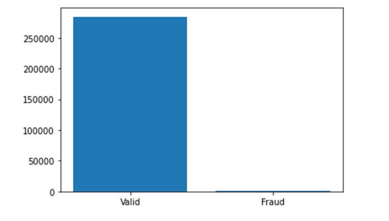
data=pd.read_csv('creditcard.csv')
plt.bar(['Valid','Fraud'],list(data['Class'].value_counts()))
print("Fraudulent transactions: ", end='')
frauds= data['Class'].value_counts()[1]/sum(data['Class'].value_counts())
print(round(frauds*100,2), end='%')
plt.show()
The dataset appears to be highly unbalanced with fraudulent transactions only representing 0.17% of all transactions. Unbalanced datasets may lead to bias in machine learning models and hence should be handled accordingly.
Determining the extent of correlations between the variables in our dataset is very useful information. This information can help with which features to extract or which machine learning model to select. Plotting the correlation matrix provides a visual summary of the correlation values between the features and the outcome.
fig=plt.figure(figsize= (12, 12))
sns.heatmap(data.corr(), cmap='Blues')
plt.show()
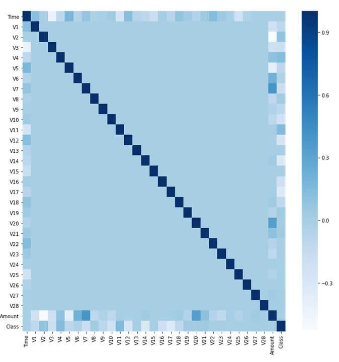
The heat-map above indicates that there are no high correlation values among the predictor columns. No predictor column has a high correlation value with the Class column either. However there exists a negative correlation among V2 and Amount as well as a positive correlation among V7 and the Amount feature.
Data Pre-Processing
Data pre-processing involves preparing the dataset to train the machine learning model. The data pre-processing step is crucial and should transform the data in a way that can be processed by the selected machine learning algorithm. For example, most classification algorithms will not be able to understand the text in the data, and hence not performing data pre-processing will lead to errors.
Common data pre-processing steps involve – imputing or dropping records containing missing values, label encoding categorical data, one hot encoding labeled data, scaling the data, and performing train-test splits on the dataset.
As this dataset does not contain any missing values or categorical data, most data pre-processing steps are not needed. The data is taken and first split into the predictors i.e. X and the outcome i.e. Y. X contains 284807 data records with 30 features each while Y contains 284807 data records with one column – class.
X =data.iloc[:,:-1]
Y =data.iloc[:,-1]
X_train, X_test, Y_train, Y_test=train_test_split(X, Y, test_size=0.2, random_state=42)
The train-test split divides the dataset into a training set and testing set. The training set is used to train the machine learning model while the testing set is used to evaluate the model. The test size of 0.2 indicates that 20% of the dataset is chosen to be the testing set. Hence, the training set contains 227845 records while the testing set contains 56962 records.
Classification Model
Selecting a machine learning model depends on the type of task that is required to be performed. Machine learning can perform various tasks such as classification, regression, clustering, pattern extraction, etc. Within each task there are a number of algorithms that may be available. Usually, two or more algorithms are experimented with to decide which model suits the data better and gives more accurate and robust results.
The credit card fraud detection problem is a classification problem, as it involves classifying a credit card transaction to be in either of the two classes – valid or fraudulent. As mentioned, there are several classification algorithms available such as Linear Classifiers, Naïve Bayes Classifier, Support Vector Machines, Nearest Neighbour Classifier, Decision Trees, etc. For this problem, a Random Forest Classifier is implemented which is an extension of the Decision Tree classifier.
classifier=RandomForestClassifier()
classifier.fit(X_train, Y_train)
Y_pred=classifier.predict(X_test)
In the above code, an object of the RandomForestClassifier class belonging to the sklearnlibrary is created. Using the fit function of this class, the model is trained using the training set. Finally, the predict function gives a prediction for the values of features in the testing set.
Model Evaluation
Every machine learning model must be evaluated on the task that it performs. Model evaluation involves asking the model to predict the values for unseen data records based on what it has learnt. This has been done above and is stored in Y_pred. Y_pred are the values as predicted by the model which must be compared against the true values i.e. Y_test. As this is a classification problem, we can evaluate the model using metrics such as accuracy, precision, and recall.
print("Model Accuracy:", round(accuracy_score(Y_test, Y_pred),4))
print("Model Precision:", round(precision_score(Y_test, Y_pred),4))
print("Model Recall:", round(recall_score(Y_test, Y_pred),4))
An accuracy of the model determines how many data records the model predicted correct values. This model has an accuracy value of 0.9996 which indicates that the model made correct predictions 99.96% of the time. Precision indicates the correctness of all those records that were predicted to be positive. A precision value of 0.963 indicates that when the model predicted a positive result it was correct 96.3% of the time. Lastly, recall of a model indicates how many truly positive values were identified correctly. A recall value of 0.7959 indicates that the model was able to identify 79.59% of all positive values correctly.
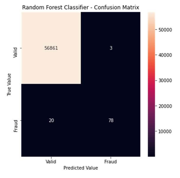
The metrics discussed above can be visualized using a heat-map on something known as the confusion matrix. A confusion matrix displays the values of the number of predictions between the true and predicted values of each class.
labels= ['Valid', 'Fraud']
conf_matrix=confusion_matrix(Y_test, Y_pred)
plt.figure(figsize=(6, 6))
sns.heatmap(conf_matrix, xticklabels= labels, yticklabels= labels, annot=True, fmt="d")
plt.title("Random Forest Classifier - Confusion Matrix")
plt.ylabel('True Value')
plt.xlabel('Predicted Value')
plt.show()
As seen from the confusion matrix, the model was correctly able to classify 56861 records as valid and 78 records as fraudulent. However, it incorrectly identified a valid transaction as a fraudulent transaction 3 times and incorrectly identified a fraudulent transaction as a valid transaction 20 times.
Therefore, in this post our machine learning classifier was able to classify the validity of credit card transactions with a 99.6% accuracy. The credit card fraud detection using machine learning is the first among the six different projects we have suggested for Data science projects for beginners, which you can explore for yourself. In case you are stuck somewhere or need further clarification on a concept, FavTutor is always here to provide you with help from expert tutors 24/7. Get started by sending a message through the chat on the bottom right. Happy programming!