When dealing with a chain of matrices, the order of multiplication can greatly impact computational efficiency. This is where the Matrix Chain Algorithm comes to the rescue. In this article, we’ll explore the Matrix Chain Algorithm, its underlying principles, and its application in optimizing matrix multiplication.
What is Matrix Chain Multiplication?
Consider a chain of matrices to be multiplied together. For example, we have matrices A, B, C, and D. The goal is to find the most efficient order of multiplication that minimizes the total number of scalar multiplications required. In this case, we can multiply them in different orders: ((AB)C)D, (A(BC))D, or A((BC)D). The Matrix Chain Algorithm helps us determine the optimal order.
The rule for matrix chain multiplication states that the order in which matrices are multiplied together can significantly impact the computational efficiency of the multiplication process. In other words, the way matrices are grouped and multiplied affects the total number of scalar multiplications required.
To illustrate this rule, consider a chain of matrices to be multiplied: A1, A2, A3, …, An. The result of multiplying this chain depends on how the matrices are parenthesized and the order in which the multiplications are performed.
For example, given matrices A, B, and C, we can have two possible ways to multiply them:
- (AB)C: In this case, we first multiply matrices A and B, and then multiply the resulting matrix with matrix C.
- A(BC): Here, we multiply matrices B and C first, and then multiply matrix A with the resulting matrix.
The rule is that the order of multiplication can affect the number of scalar multiplications required to obtain the final result. In some cases, different parenthesizations can lead to significantly different numbers of scalar multiplications.
For instance, the number of scalar multiplications required for the product (AB)C can be fewer than the number required for A(BC). The rule emphasizes that the order of multiplication should be chosen in a way that minimizes the total number of scalar multiplications in order to optimize the matrix chain multiplication process.
Matrix Chain Multiplication Example
Let’s consider an example to illustrate the matrix chain multiplication.
Suppose we have a chain of four matrices: A, B, C, and D, with dimensions as follows:
A: 10 x 30
B: 30 x 5
C: 5 x 60
D: 60 x 8
The goal is to find the optimal order of multiplying these matrices that minimizes the total number of scalar multiplications.
To solve this problem, we can apply the Matrix Chain Multiplication algorithm using dynamic programming. Let’s go step by step:
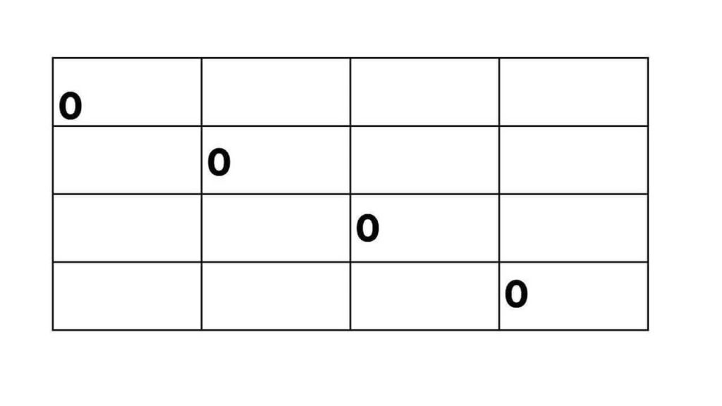
Step 1: Create the table We create a 4×4 table to store the minimum number of scalar multiplications needed for each subchain. The table initially looks like this:
Step 2: Fill in the table We iterate diagonally through the table, calculating the minimum number of scalar multiplications for each subchain.
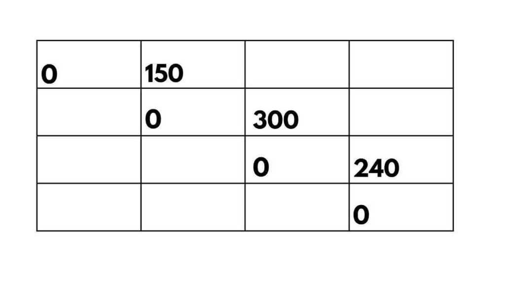
First, we consider subchains of length 2: For the subchain AB, the only option is multiplying matrices A and B, resulting in 10 x 5 scalar multiplications. For the subchain BC, the only option is multiplying matrices B and C, resulting in 30 x 5 scalar multiplications. For the subchain CD, the only option is multiplying matrices C and D, resulting in 5 x 8 scalar multiplications.
Updating the table:
Next, we consider subchains of length 3: For the subchain ABC, we have two options: (AB)C or A(BC). Let’s calculate the scalar multiplications for each option:
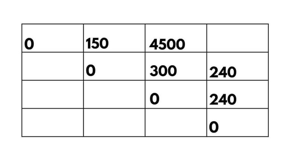
- (AB)C: We multiply matrices A and B (10 x 30) resulting in a temporary matrix of size 10 x 5. Then, we multiply this temporary matrix with matrix C (10 x 5) resulting in a final matrix of size 10 x 60. The total scalar multiplications for this option are 10 x 30 x 5 + 10 x 5 x 60 = 4500.
- A(BC): We multiply matrices B and C (30 x 5) resulting in a temporary matrix of size 30 x 60. Then, we multiply matrix A (10 x 30) with this temporary matrix, resulting in a final matrix of size 10 x 60. The total scalar multiplications for this option are 10 x 30 x 60 + 10 x 5 x 60 = 9000.
Updating the table:
Finally, we consider the entire chain of matrices ABCD: We have two options: ((AB)C)D or (A(BC))D. Calculating the scalar multiplications for each option:
- ((AB)C)D: We multiply matrices (AB) and C, resulting in a temporary matrix of size 10 x 60. Then, we multiply this temporary matrix with matrix D (10 x 60), resulting in a final matrix of size 10 x 8. The total scalar multiplications for this option are 10 x 5 x 60 + 10 x 60 x 8 = 6000.
- (A(BC))D: We multiply matrices A and (BC), resulting in a temporary matrix of size 10 x 60. Then, we multiply this temporary matrix with matrix D (10 x 60), resulting in a final matrix of size 10 x 8. The total scalar multiplications for this option is 10 x 30 x 5 + 10 x 5 x 8 = 1300.
Updating the table:
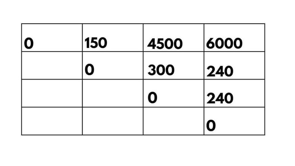
Step 3: Backtrack the optimal solution To determine the optimal order of multiplication, we start at M[1, 4], which gives us the minimum number of scalar multiplications for the entire chain. In this case, M[1, 4] = 6000, indicating that ((AB)C)D is the optimal order.
Step 4: Return the result The minimum number of scalar multiplications required to multiply the entire chain is 6000, and the optimal order is ((AB)C)D.
That’s an example of how the Matrix Chain Multiplication algorithm works. By applying dynamic programming, we can find the optimal order and minimize the computational cost of multiplying a chain of matrices.
Algorithm to Solve Matrix Chain Multiplication
The matrix chain multiplication algorithm is a dynamic programming approach used to determine the most efficient order of multiplying a chain of matrices. It aims to minimize the total number of scalar multiplications required to compute the final matrix product.
Let’s break down the steps of the algorithm:
- Define the problem:
- Given a chain of matrices A1, A2, A3, …, An, where the dimensions of matrix Ai are d[i-1] x d[i] for i = 1 to n.
- The goal is to find the optimal order of matrix multiplication to minimize the total number of scalar multiplications.
- Create a table:
- Create an n x n table, where n is the number of matrices in the chain.
- The table, let’s call it M, will store the minimum number of scalar multiplications required to multiply the subchains of matrices.
- Initialize the table:
- Set the diagonal entries of M to 0, as the subchains of length 1 do not require any multiplication.
- Fill in the table:
- Iterate over the table diagonally, starting from the subchains of length 2 and gradually increasing the length.
- For each subchain length k, starting from matrix i, calculate the minimum number of scalar multiplications.
- For each possible split point j, where i ≤ j < i + k, calculate the number of scalar multiplications as follows:
- Compute the number of scalar multiplications required for the left subchain: M[i][j]
- Compute the number of scalar multiplications required for the right subchain: M[j+1][i+k]
- Calculate the number of scalar multiplications for the current split point: d[i-1] * d[j] * d[i+k] + M[i][j] + M[j+1][i+k]
- Update the table entry M[i][i+k] with the minimum value among all possible split points.
- Backtrack the optimal solution:
- To determine the optimal order of matrix multiplication, track the split that gives the minimum number of scalar multiplications for each subchain.
- This can be achieved by storing additional information during the table-filling step, such as the split points that yield the minimum number of scalar multiplications for each subchain.
- Return the result:
- The minimum number of scalar multiplications required to multiply the entire chain is stored in M[1][n], where n is the number of matrices in the chain.
- The optimal order of matrix multiplication can be obtained by backtracking through the split points stored during the algorithm execution.
Here’s a pseudo-code representation of the matrix chain multiplication algorithm:
function matrixChainMultiplication(dimensions):

   n = length(dimensions) - 1

   create an n x n table M

   for i = 1 to n:

       M[i][i] = 0

   for length = 2 to n:

       for i = 1 to n - length + 1:

           j = i + length - 1

           M[i][j] = infinity

           for k = i to j - 1:

               cost = M[i][k] + M[k+1][j] + dimensions[i-1] * dimensions[k] * dimensions[j]

               if cost < M[i][j]:

                   M[i][j] = cost

   return M[1][n]
C++ Program
Here’s an implementation of the matrix chain multiplication algorithm in C++:
#include <iostream>

#include <climits>

using namespace std;

int matrixChainMultiplication(int dimensions[], int n) {

   int dp[n][n];

   for (int i = 1; i < n; i++) {

       dp[i][i] = 0;

   }

   for (int length = 2; length < n; length++) {

       for (int i = 1; i < n - length + 1; i++) {

           int j = i + length - 1;

           dp[i][j] = INT_MAX;

           for (int k = i; k < j; k++) {

               int cost = dp[i][k] + dp[k + 1][j] + dimensions[i - 1] * dimensions[k] * dimensions[j];

               if (cost < dp[i][j]) {

                   dp[i][j] = cost;

               }

           }

       }

   }

   return dp[1][n - 1];

}

int main() {

   int dimensions[] = {10, 30, 5, 60};

   int n = sizeof(dimensions) / sizeof(dimensions[0]);

   int minimumMultiplications = matrixChainMultiplication(dimensions, n);

   cout << "Minimum number of scalar multiplications: " << minimumMultiplications << endl;

   return 0;

}Output:
Minimum number of scalar multiplications: 4500
Time and Space Complexity
The time complexity of the algorithm is determined by the nested loops used to fill in the dp table. The outer loop iterates from length = 2 to n, and the inner loops iterate from i = 1 to n – length + 1 and k = i to j – 1. Therefore, the total number of iterations is roughly proportional to the sum of the arithmetic series from 2 to n, which can be simplified as O(n^3). Hence, the time complexity of the code is O(n^3).
The space complexity of the code is determined by the dp table, which is an n x n matrix. Therefore, the space required to store the dp table is O(n^2). Additionally, the space complexity of the code is further influenced by the input array dimensions[], which have a size of n. Therefore, the overall space complexity of the code is O(n^2).
Applications
The matrix chain multiplication algorithm has several applications in various fields. Some of the common applications include:
- Computer Graphics: In computer graphics, matrix transformations are used to perform operations like scaling, rotation, translation, and projection. Matrix chain multiplication is utilized to optimize the order of these transformations, reducing the computational overhead and improving rendering performance.
- Image and Video Processing: Matrix operations are frequently employed in image and video processing algorithms, such as filtering, compression, and feature extraction. Matrix chain multiplication helps optimize the sequence of operations, enabling efficient processing of large amounts of image or video data.
- Optimization Problems: Matrix chain multiplication can be used to solve optimization problems, such as finding the optimal sequence of actions or operations. Examples include scheduling problems, production planning, resource allocation, and network optimization, where matrices represent different tasks or operations, and the goal is to minimize the overall cost or time.
- Robotics and Motion Planning: Matrix transformations play a vital role in robotics for calculating the kinematics and dynamics of robotic systems. Matrix chain multiplication is utilized to optimize the order of transformations and computations involved in motion planning, inverse kinematics, and trajectory generation.
- Algorithm Design and Analysis: The matrix chain multiplication problem is often used as a benchmark in algorithm design and analysis. It serves as an example of dynamic programming, highlighting the importance of optimizing subproblems to solve larger-scale problems efficiently.
- Computational Biology: Bioinformatics and computational biology involve analyzing large datasets of biological sequences, such as DNA and protein sequences. Matrix chain multiplication can be applied to optimize sequence alignment algorithms, phylogenetic tree construction, and other sequence analysis tasks.
- Data Science and Machine Learning: Matrix operations are fundamental in data science and machine learning. Matrix chain multiplication can be used to optimize the computation of matrix factorization, dimensionality reduction, clustering, and deep learning algorithms, improving computational efficiency and training speed.
- Parallel and Distributed Computing: Matrix chain multiplication algorithms can be parallelized and distributed across multiple processors or computing nodes. This allows for efficient utilization of resources, reducing computation time and improving overall system performance in parallel and distributed computing environments.
Conclusion
In this article, we learned how to solve the Matrix Chain Multiplication problem using Dynamic Programming. It is a fundamental operation in various fields, including computer graphics, scientific computing, and machine learning.

