In the context of data structures and algorithms, the real-life scenario of when to buy and sell stocks for Profit maximization in stock trading can be framed as a problem. In this article, we will learn about the “Best Time to Buy and Sell Stock II” problem is an extension of the famous problem “Best Time to Buy and Sell Stock”, which can be solved with the help of dynamic programming.
Best Time to Buy and Sell Stock II Problem
In the famous leetcode problem to find the best time to buy and sell stock, we are given daily stock prices in an array, the task is to maximize profit through strategic buying and selling decisions.
We can buy and sell on the same day. We have to analyze the array to identify optimal transactions and to return the maximum achievable profit in this stock trading scenario. For example:
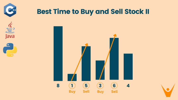
Input: prices = [8,1,5,3,6,4]
Output: 7
Buy on day 2 (price = 1) and sell on day 3 (price = 5), profit = 5-1 = 4. Then buy on day 4 (price = 3) and sell on day 5 (price = 6), profit = 6-3 = 3. Total profit is 4 + 3 = 7.
The following guidelines need to be followed:
- To sell the stock, we must first buy it on the same or any previous day.
- We can buy and sell the stock any number of times.
- We first buy a stock and then sell it. After selling we can buy and sell again. But we can’t sell before buying and can’t buy before selling any previously bought stock.
Recursive Approach
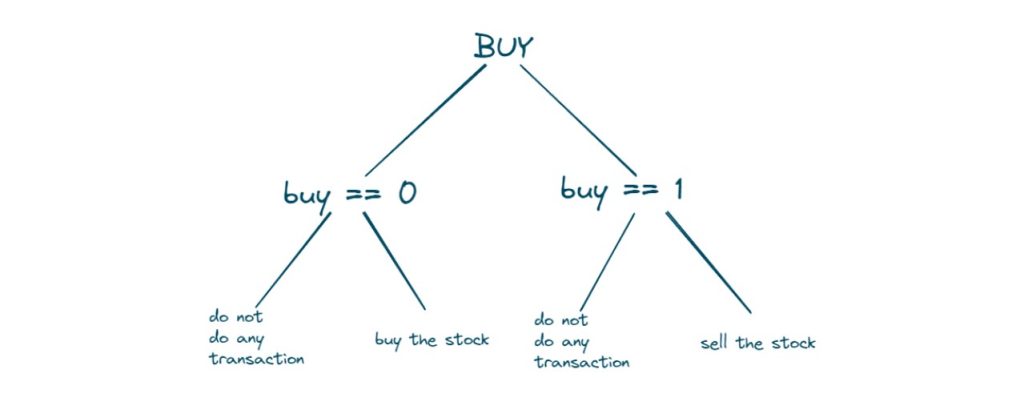
As in this problem, we can buy and sell stocks multiple times and we have to maximize profit so we have to explore all possibilities, i.e. On each day we have two choices either to do nothing and move to the next day or to buy/sell (based on the last transaction) and find out the profit. We can solve it using recursion easily.
So to start our recursive solution we need to express our problem in terms of index: We will start from day 1 and will go to the last day exploring all possibilities of each index based on the previous transaction.
Here are the steps to be performed for recurrence relation:
- We will start from day 1 and declare a buy variable that tells us on a particular day whether we can buy or sell the stock.

- Every day we have two choices to either buy/sell stock based on previous transactions or to do nothing and move on to the next day.
Case 1:
When buy == 0 where we can buy stock on a particular day so we have 2 options
- To skip the transaction and go on to the following day:
- Since there will be no net profit from the current transaction, we will call f(ind+1,0) recursively to determine the maximum profit that may be made beginning on the next day.
- The ‘buy’ variable value will remain at 0, meaning that we can purchase the stock the following day, since we haven’t purchased it yet.
- If we decide to buy the stock on a particular day, it means we are choosing an alternative option.
- In this case, the profit we gain will be negative, represented by -Arr[i].
- This happens because we use our own money to buy the stock.
- The profit becomes zero since we are essentially spending our cash. By making a recursive call to f(ind+1,1), we figure out the best profit starting from the next day.
- Once we buy the stock, the “buy” variable becomes 1, indicating that we can’t buy it again and must sell it the following day
Case 2:
When buy == 1 where we can sell previously bought stock
- Choosing not to make any transaction means moving to the next day.
- In this situation, the profit earned from the current transaction is zero.
- To find the maximum profit from the next day onward, we use a recursive call to f(ind+1,1).
- Since we haven’t purchased the stock, the ‘buy’ variable stays at 1, signaling that we can only sell the stock the following day and cannot make another purchase.
- Another choice is to sell the stock in the present day.
- Here, the profit gained from the current transaction is +Arr[i].
- Since we are selling the stock, we are receiving money, resulting in a positive profit.
- To find the highest profit starting from the next day, we use a recursive call to f(ind+1,0).
- After selling the stock, the ‘buy’ variable switches to 0, signalling that we can purchase the stock the following day.

To return maximum profit we have to take the maximum value of both cases. If ind==n, we simply return 0 because it indicates that we have completed trading on all days and that there is no more money available.
The worst-case time complexity of the recursive solution is exponential, O(2^n), where n is the number of days or the size of the input array.
The space complexity is linear, O(n), where n is the number of days or the size of the input array. This is because the space required by the call stack is directly related to the number of recursive calls, which, in turn, is determined by the number of days.
Dynamic Programming Approach
To optimize the recursive solution, we observe overlapping subproblems and introduce a dynamic programming approach:
- Create a 2D array named dp with dimensions [n][2], where ‘n’ is the size of the input array. This array will store solutions for subproblems and Initialize the dp array with -1.
- When calculating a solution for specific parameters (e.g., f(ind, buy)), first check if it’s already computed using the dp array (i.e., dp[ind][buy] != -1).
- If the solution is already available, return the stored value from the dp array.
- If not, compute the solution using the standard recursive relation. Before exiting the function, update dp[ind][buy] with the calculated solution.
- This dynamic programming approach helps avoid redundant calculations by storing and reusing previously computed results, enhancing the efficiency of the solution.
C++ Code
Here is the C++ program that uses dynamic programming approach:
#include <iostream>
#include <vector>

using namespace std;

int help(int ind, int buy, vector<int>& prices, vector<vector<int>>& dp) {
    if (ind == prices.size())
        return 0;

    int profit = 0;

    if (dp[ind][buy] != -1)
        return dp[ind][buy];

    if (buy) {
        profit = max((-prices[ind] + help(ind + 1, 0, prices, dp)), help(ind + 1, 1, prices, dp));
    } else {
        profit = max((prices[ind] + help(ind + 1, 1, prices, dp)), help(ind + 1, 0, prices, dp));
    }

    return dp[ind][buy] = profit;
}

int maxProfit(vector<int>& prices) {
    vector<vector<int>> dp(prices.size() + 1, vector<int>(2, -1));
    return help(0, 1, prices, dp);
}

int main() {
    vector<int> prices = {8, 1, 5, 3, 6, 4};

    // Call the maxProfit function and print the result
    cout << "The maximum profit that can be generated is " << maxProfit(prices) << endl;

    return 0;
}
Java Code
Here is the solution in Java:
import java.util.Arrays;

public class StockProfit {

    static int help(int ind, int buy, int[] prices, int[][] dp) {
        if (ind == prices.length)
            return 0;

        int profit = 0;

        if (dp[ind][buy] != -1)
            return dp[ind][buy];

        if (buy == 1) {
            profit = Math.max((-prices[ind] + help(ind + 1, 0, prices, dp)), help(ind + 1, 1, prices, dp));
        } else {
            profit = Math.max((prices[ind] + help(ind + 1, 1, prices, dp)), help(ind + 1, 0, prices, dp));
        }

        return dp[ind][buy] = profit;
    }

    static int maxProfit(int[] prices) {
        int n = prices.length;
        int[][] dp = new int[n + 1][2];
        for (int[] row : dp) {
            Arrays.fill(row, -1);
        }
        return help(0, 1, prices, dp);
    }

    public static void main(String[] args) {
        int[] prices = {8, 1, 5, 3, 6, 4};

        // Call the maxProfit function and print the result
        System.out.println("The maximum profit that can be generated is " + maxProfit(prices));
    }
}
Python Code
You can implement it in Python as well:
def help(ind, buy, prices, dp):
    if ind == len(prices):
        return 0

    if dp[ind][buy] != -1:
        return dp[ind][buy]

    if buy:
        profit = max((-prices[ind] + help(ind + 1, 0, prices, dp)), help(ind + 1, 1, prices, dp))
    else:
        profit = max((prices[ind] + help(ind + 1, 1, prices, dp)), help(ind + 1, 0, prices, dp))

    dp[ind][buy] = profit
    return profit

def max_profit(prices):
    n = len(prices)
    dp = [[-1] * 2 for _ in range(n + 1)]
    return help(0, 1, prices, dp)

if __name__ == "__main__":
    prices = [8, 1, 5, 3, 6, 4]

    # Call the max_profit function and print the result
    print("The maximum profit that can be generated is", max_profit(prices))
Output:
The maximum profit that can be generated is 7The time complexity is O(N*2) because there are N*2 states therefore at max ‘N*2’ new problems will be solved and we are running a for loop for ‘N’ times to calculate the total sum. The Space Complexity is O(N*2) + O(N) because We are using a recursion stack space(O(N)) and a 2D array ( O(N*2)).
Here is brief comparison of both the approaches:
| Approach | Time complexity | Space complexity | Details |
| Recursive Approach | O(2^N) | O(N) | Because the number of recursive calls at each level of the tree doubles, leading to an exponential growth in the number of total calls. |
| Dynamic programming Approach | O(N*2) | O(N*2) + O(N) | There are N*2 states therefore at max ‘N*2’ new problems will be solved and we are running a for loop for ‘N’ times to calculate the total sum. |
Conclusion
In Conclusion, the Best Time to Buy and Sell Stock II leetcode problem can be easily solved using a recursive approach and it can be further optimized by using Dynamic Programming. It is one of the most asked problems in the interviews.


